Pinholes and pinheads! Before getting to the latest installment of the Calibration Campaign, I want to remind everyone that I welcome questions and comments (unless you are a troll!). Happy to answer. Also do hit the subscribe button so you never miss a post; and please tell your friends!
With that, on to the latest. Last week, I ran to tests to help me figure out how the system is behaving. And by “the system” I include both the hardware (microscope and gizmos) and the biology (xylem stained to light up cellulose).
The first test was to check how the calibration is doing. I followed a suggestion of Rudolf Oldenbourg, who has been helping me get this all working. I imaged the edge of a polarizing filter (Fig. 1). I chose the edge to be parallel to the transmission axis of the filter. This provides a kind of ground truth to which way the light is polarized. I captured images as if I were using fluorescence: in this case, the software calculates the orientation of maximum transmission rather than fluorescence emission. The math is the same. I rotated the filter by ~15º and captured again. I covered about 180º.

Figure 1. Transmitted light image of the edge of a polarizing filter. The transmission axis of the filter (double red arrow) is parallel to the edge. I measured the angle calculated by the system in a large region (red triangle), well away from the distortions near the edge.
Physically, this was harder than it sounds because I am using a water immersion lens. I taped a coverslip to hang way over the edge of a slide. I immersed the objective onto the coverslip and then, gently, placed the polarizing filter on the coverslip so that the filter’s edge was in the field of view. Hey presto!
With the images saved, I measured the angle the edge makes with the horizontal, which I will call the reference angle, and which reflects the known transmission axis of the filter. I then obtained the orientation of the transmission axis as calculated by the software. Plotting these shows how well the system is calibrated (Fig. 2).

Figure 2. Calibration check. The reference angle is my best estimate of the direction of the edge (double arrow in Fig. 1). Calculated angle is that found by the software.
And how well *is* the system calibrated? I am not sure. From far away, the points are not so far from falling on the line (the solid, diagonal line of 1:1, perfect calibration). But from closer up, anomalies are clear. The points around 45 and 135º are around 10º off, and there is some funny biz going on around 170º. I don’t know if I can hone the calibration any finer. I am going to make this curve again using a cleaner way to rotate the polarizing filter, see if that weirdness at 170º is real. But maybe this is as good as it gets?
The next test I did centered on the test sample (Fig. 3). In general, I want to measure the angle of a stained xylem rib directly and then compare that to the angle calculated by the software (this is same kind of test as described above for the edge of the polarizing filter only now done in fluorescence). But I decided to add on top of that a further test because it will take a large paragraph to explain to you. Here goes.

Figure 3. Fluorescence image of celery xylem stained with fast scarlet. This image was taken with the pinhole set to 0.5 AU. An “AU” stands for an Airy unit, which is an optical criterion based on the limit of resolution in the image plane.
In my last post, I wrote about the possibility of distortions to the calculations arising from the sample’s auto-fluorescence. Now I am working at 561 nm, a longer wavelength that induces much less auto-fluorescence. But there is another way that the sample could be interfering. The ribs in the figure are the tips of a xylem-berg, I mean those ribs overlie several other strands as well as collapsed intervening parenchyma, which also contains cellulose. The confocal optics are designed to reject all this out-of-focus signal originating from beyond the focal plane; but, the rejection is hardly perfect. The rejection depends on light passing through a pinhole. In effect, the pinhole generates a tiny probe to raster over the sample, rather than the broad beam of the entire objective. The software allows me to vary the diameter of the pinhole. The smaller the pinhole, the less out-of-focus light and conversely, the larger the pinhole, the more. I reasoned that I could spot interference from the underlying sample if any discrepancy between the measured and calculated angles of a rib got larger with pinhole diameter.
I imaged the ribs in figure 3 four times, changing only the pinhole diameter. Then, for each of 28 ribs, I measured the angle of the rib to the horizonal manually (reference) and then obtained the angle calculated for that rib by placing a region of interest over the rib in question. I used the identical region for the four pinhole diameters (Fig. 4).

Figure 4. Xylem rib check. For the xylem shown in Figure 3, I measured the angle manually (“reference”) and compared this to the angle calculated by the software based on the apparent anisotropy of fluorescence. I did this for 28 ribs (“xylem rib ordinal”). The colored open circles show results for the same cell imaged with various pinhole diameters.
Clearly, the pinhole matters, but only when it is big (Fig. 4, red circles: 4 AU). For the usual pinhole size (1 AU) cutting the diameter by half or doubling it makes little difference in the calculated angle. So at least for this this object, the confocal optics are doing their job.
But as the reference angle goes from ~135º towards 90º, a discrepancy looms. The points for the reference angle (black circle) and the calculated angles (colored circles) diverge. Much as I’d like to, I cannot blame this divergence on dark matter, I mean out-of-focus signal. I plotted the discrepancy versus the reference angle (Fig 5). Wow! A straight line. And down around 90º, these discrepancies are embarrassingly large.
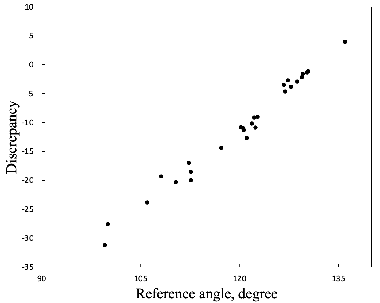
Figure 5. A line in the sand. In the plot, “discrepancy” is the difference between the reference angle and the calculated angle (for 0.5 AU) for the data in Fig. 4.
I feel this linear relationship squarely implicates the hardware. Can I shrink the discrepancy by better calibration? How influential will the background correction turn out to be? The line is drawn.
Hi Tobias,
Nathanael here from Sheffield. I stumbled on your blog while researching calcofluor polarization and have been following with rapt attention. A system like this would be a dream to work on and it’s been incredibly insightful watching your process of systematically ironing out kinks and problems.
The deviations in your dry (polarized film) calibrations are suspiciously systematic – sigmoidal, in fact. Are you using the same edge of the filter to calibrate each time? In Figure 1 I see what looks like the ‘shadow’ of the bottom edge of the filter some distance from the upper edge. I can’t quite picture it but perhaps this is throwing things off somehow.
Another fringe possibility relates to scanfield rotation. You’ve probably seen Thomas et al. (doi: 10.1111/jmi.12582) who modulate laser polarisation with scanfield rotation. If I had understood correctly, this effect is most prominent at 405 nm and drops off for 561 nm; furthermore they report that this only works for specific microscopes. We have an LSM 880 and I have tested this very perfunctorily and it seems not to matter, so perhaps this is a red herring – but potentially worth verifying and it should be easy enough to switch the scanfield in ZEN unless the PolScope software gets in the way.
Figure 5 is very interesting – how does a discrepancy plot look like
for the data in Figure 1? (conversely how do the data from Figure 4 look like slotted into Figure 1?) My impression is that in this case the discrepancy is reversed, starting pretty good at 90 and getting much worse at 135.
One final thing – I wonder if the cellulose microfibrils are definitely aligned perfectly along the long axis of the ribs. The AFM from Gray Cellulose (2014) you mentioned is not particularly convincing, and for the fibres to pitch and twist in the manner they do, perhaps they are doing someting subtle with their orientation.
This could all be wrong and I’m sure you’ve made great progress by now – just wanted you to know that at least one more person is out there is following very keenly!
Nat, Thank you for your thoughtful comment. Wonderful to hear of your interest. Actually I hadn’t known of that scanfield thing. I am going to look it up directly. Yes, you are right that the test with polarizing filter is a little sketchy and I need to repeat. I have thought of a way to do it more easily and that should help. You are also right to notice that the curve for the calibration test in transmitted light seems to be out where the curve from the xylem ribs is in. But I have a nother xylem where the match is perfect at 90 degrees and out with distance away. I have made a prep that I can rotate which should let me look at the same ribs as they are rotated. And finally, also yes, the substructure of the xylem rib could indeed be more complex than I am giving credit. Previously I used BY-2 cell xylem, which are young and simple. We can check this with birefringence. Its a good idea.