
by Ryan Wicks | Summer 2023
Introduction
For decades aircraft and spacecraft technologies have been leveraged in agriculture. For aircraft applications, aerial crop dusting might come to mind, and I include spacecraft technologies for at least two roles that they play: for one they are used for remote sensing in a variety of applications, some of which collect information on environmental conditions that impact agriculture as well as collecting information on soil or vegetation health on farmland; secondly they are used indirectly to assist in navigation of other survey tools and automated fertilizer or pesticide application systems. With the proliferation of unpiloted aircraft systems (UASs), or “drones”, these technologies have been added to tools that can be leveraged in agriculture. While they have been adopted at different rates and in different ways for agriculture in different parts of the world in the past couple of decades, there seems to be a definitive niche for their use in some way or another in agriculture, though that niche varies depending on the geological region and what kind of agriculture they are being used to support.
Agricultural applications of drones are not my own focus area, but for some of my colleagues it is the primary focus of how they think about leveraging drones, and certainly I have not been entirely absent from using UAS and survey tools in support of agricultural applications. While I could talk in detail about any number of theses agriculture-related projects, in this article I want to give a brief overview of how different teams at UMass have leveraged more advanced survey tools like UAS and RTK GNSS in support of their work.
UMass Agricultural Learning Center
The University of Massachusetts operates several different farms in support of research or education, one such farm is located just north of the core Amherst campus. We’ve been teaching UAS applications for 7 years now, and as part of the curriculum we ask students plan and conduct surveys using drones. The field at the UMass Agricultural Learning Center (https://www.umass.edu/stockbridge/student-life/umass-agricultural-learning-center) has been a location that has been surveyed three times now as a final project for a class, and the main focus for students working on these projects has been to produce accurate high-resolution orthomosaics and digital elevation models (DEMs). The latter is particularly useful for producing flood-routing maps for locating erosion patterns – a workflow that was suggested and explored in a few different ways by a variety of students. The first team, Jason Roach and Vincent von Dosky, surveyed the Agricultural Learning Center in the Spring of 2018, and a second team, Peter Crump and Timothy Fistori, surveyed the site in the Spring of 2022. In 2021 another team comprised of Caleb Zimmerman and Jake Butler, did their own reconstructions and analysis of derivative orthomosaics and elevation models from the images that were collected in 2018. Each team produced a digital elevation model (DEM) that was accurate to within several centimeters and used that model to develop slope or gradient models and flood routing models. The two surveys that were done were separated by 4 years, and as such can hypothetically be used to understand changes in the topology and flood routing if the data is accurate enough. Both surveys were done using GCPs, and so their accuracy is substantial enough to enable a variety of different analyses. The student teams generally conducted analysis of the elevation models to create models of flood routing or general hydrology using a variety of GIS tools. While I do not have the specific files each team used, I have taken the raw images and GCP data to reconstruct the elevation models of the fields in 2018 and 2022 respectively, and have recreated the general type of workflow that the student teams developed to study the topography and flood routing. While the workflow that I talk about here is specifically different than what any one team did for analysis, and although it is perhaps most representative of the specific procedure that Peter Crump and Timothy Fistori developed, though all teams developed and explored a workflow that aimed to be at least conceptually similar though not exactly what is shown here.


I want to talk a little bit about how these flood routing channel networks are predicted and modeled, as well as why this might be significant or useful information. As I explain the methodology I want to focus on the model that was produced from the 2022 imagery and photogrammetry-derived elevation model. I think Dr. Hans van der Kwast, a lecturer from IHE Delft Institute for Water Allocation, does a good job of providing an overview of the theory of each of the steps to develop channel network models and catchment basin models in this video: https://www.youtube.com/watch?v=ZLUjSEK-nbg&list=PLeuKJkIxCDj2Gk0CkcJ-QeviE41aMZd-5. This is part of his open course on GIS, and he uses tools from the PCRaster package; although we didn’t use those specific steps, the theory presented in his video is applicable to the specific approach and steps I discuss here. I used the SAGA 7.8.2 tool library to recreate what some of the students did for their analysis, and the specific procedure I followed is covered in this tutorial provided by Hatari Labs: https://www.youtube.com/watch?v=jiREWrkHjs8. SAGA 7.8.2 source code can be found at https://github.com/qgis/QGIS/issues/46837, though it can be installed as part of the primary QGIS install; I used QGIS 2.28.9-Firenze. Documentation on the SAGA tool library can be found here: https://saga-gis.sourceforge.io/saga_tool_doc/index.html.


We used the QGIS SAGA tool “Channel Network and Drainage Basins”. Figures 1g-1l highlight some of the higher-level steps that the tool takes to compute the channel network as well as shows some of the products produced from using this tool.


I have written about the importance of using ground control points (GCPs) before, and there is a similar level of importance to using ground control points in agriculture. While accuracy is nice to have, at the very least maintaining precision is of particular importance, even when higher accuracies are not available. Simply by placing markers in a field or fields that are going to be surveyed using a drone will help considerably. In the case of modeling the UMass Agricultural Center, if the same markers had been placed in a stable location and not moved significantly over the several years that passed between surveys, the same markers could be referenced in both surveys to maintain consistency of precision and so that the data layers produced at both times would align within a few centimeters of each other, even if the makers were never surveyed relative to some datum like the 1983 North American Datum (NAD 83). Though no long-term markers were placed, however, each team did place temporary markers and did survey their respective locations with an R10 RTK GNSS receiver so that not only could a higher precision be achieved, but a higher accuracy as well, on the order of a few centimeters. This allows the analysis over time to be much more reliable, and to account for any potential shift in the GCP markers. In some environments, such as in salt marshes where I usually do most of my surveying, the peat can expand and contract or shift considerably from season to season, and so it is important to survey the GCP markers at least every year if we want to maintain a higher level or accuracy.
Lettuce Project
Just another ten miles or so north of the Student Ag Center is another research and education farm that UMass operates in South Deerfield. A few years ago I worked with Dr. Omidreza Zandvakili to explore the use of UAS to detect and measure the effect of varying fertilizer applications on the growth and health of lettuce. We had placed GCPs and surveyed them using an R10 unit and then collected 5-band multispectral imagery using a Micasense RedEdge-M camera mounted on a DJI Matrice 600. In general, orthomosaics and DEMs are data sets that are spatially-related data, and any time one wants to do analysis that leverages those data products as part of a process that calls for such a higher level of accuracy, possibly incorporating other data sets that are spatially-related and have a certain degree, it is important to have a similar level of accuracy. As it turns out those data products that we produced from those surveys and flights didn’t end up being analyzed in relation to any other high-accuracy data sets, but potentially if the scope of the project had called for repeated surveying, we certainly could have benefited from having the accuracy and precision afforded by having surveyed GCPs.
When Dr. Zandvakili conducted the analysis for the study interestingly no significant change in NDVI was found between batches of lettuce that had varying levels of fertilizer applied to them, however, there did appear to be significant difference in the size of the lettuce plants between batches which had varying levels of fertilizer application. The high-resolution images and elevation models were sufficient to delineate the approximate lateral boundary of each lettuce head, as well as to measure the elevation within this boundary; thus the volume could also be calculated by integrating the elevation values across the boundary. While high-precision was required for this particular operation, high accuracy was not strictly necessary and thus the GCPs were not strictly necessary, though they did help improve the precision to a degree. Had these measurements of the lettuce head been needed to be measured at various points over longer time scales then the use of GCPs to achieve higher accuracy would have been more useful.

Fig. 2a – Here is a section of a Red-Green-Blue (RGB) orthomosaic that was produced by flying over the plots of lettuce in Dr. Zandvakili’s study. The image is oriented so that the north direction is towards the top of the image. You may note that the western plots were weeded regularly while the eastern plots were not. One of the GCPs that was used is visible in the north-west corner of this image of the field.

Fig. 2b – This shows the same region but with color scale applied to the Normalized-Difference Vegetation Index (NDVI). The NDVI helps indicate the relative stress of plants, and can also be used to delineate vegetation from the background. You may note that the lettuce heads are more clearly defined where there is not an abundance of weed vegetation.

Fig. 2c – This shows the same region but as an image that shows elevation represented in grayscale. The volume of each lettuce head can be calculated by integrating within the boundary of the lettuce head the elevation of each pixel relative to the mean elevation of the boundary of the elevation of each lettuce head. The boundary can be defined in several ways. The most basic method is by human photointerpretation, but in this case the NDVI or DEM itself could be delineated using some basic delineation algorithms on QGIS, such as the “Polygonize” tool, to find the boundary of the lettuce heads.
Cranberry Bog LWIR Surveys
Among the many other projects taking place at the UMass Cranberry Station in East Wareham, MA are a series of projects to explore the adoption of drone technologies to improve precision of cranberry agriculture. Cranberries are one of the most prolific crops grown in Massachusetts, and multiple cranberry farms have begun to adopt drones in a variety of capacities, including scouting for crop damage and fertilizer and pesticide applications. At the Cranberry Station Dr. Giverson Mupambi is one of the researchers exploring the use of drone technologies and different ways they might be applied to for scouting and monitoring vegetation health and conditions on a cranberry farm. One novel approach that is to use a drone equipped with a long-wave infrared (LWIR) to scout for potential frost damage.
Cranberry plants do not shed their leaves in the winter, but rather the plant and its leaves enter a dormant stage where the plant’s leaves turn from green to a deep purple or maroon color. The cranberry leaves accumulate anthocyanin which allows it to tolerate colder temperatures below freezing. Towards the end of the winter as the season transitions to spring, gradually the plants come out of dormancy and they start to diminish their frost-resistant properties. Coming out of dormancy too late means missing some of the growing season, coming out of dormancy too early means risking frost damage. The plants regulate this process themselves naturally, but they are still in general vulnerable to frost damage at certain points, and if the temperature drops too low on a particular night there could be significant damage to the crop and the prospects for harvest later that year. Farmers have the ability to mitigate frost damage by using their irrigation systems to spray water on the plants overnight to keep the temperature at around a freezing temperature, which is usually still several degrees above what the plants can tolerate towards the end of the winter. Running the irrigation has costs, however, and typically farmers will try to limit how much they leverage the irrigation as a tool to mitigate frost by only using it if the temperature drops below a certain temperature threshold. That temperature threshold becomes higher and higher as the plants come further and further out of dormancy. Typically farmers will place a temperature logger on the cranberry bog platform somewhere to monitor the temperature.
Selecting the ideal location, however, is not obvious and is important. An older technique is to see where mist settles most quickly or thickly on a bog surface as temperatures cool. Dr. Mupambi suggested that LWIR surveys using drones late in the winter could be used to see the range of temperatures that exist on a cranberry bog surface, as well as what the distribution of temperature is over the surface of a bog and where the coldest temperatures are. Having conducted an initial test at the Cranberry Station last year, we found that the difference between the minimum and maximum temperature on the bog was about 6.7 degrees Celsius, or about 12 degrees Fahrenheit. As Fig 3c shows, we located roughly the coldest spot on the bog, and then looked at the distribution of temperatures within 5 meters of that location. If one wanted to place a temperature probe on the bog to monitor for temperatures that get low enough to justify the use of irrigation to mitigate against frost damage, one might want to place the temperature probe at the coldest location on the bog surface. In this instance the use of GCPs can help locate the coldest location accurately, and an RTK GNSS receiver can help guide the placement of a temperature probe more accurately. Without such accuracy, it is quite possible that the probe could be placed 5-10 meters from the intended location. While in many cases the temperature probably doesn’t vary too much over this distance, as we showed in this one simple test it seems that it may be possible that temperatures vary by as much as 3.7 degrees Celsius within a 5 meters radius of a given location on the bog. In this particular test we were just trying to demonstrate a proof of concept for a workflow, so we did not use GCPs, but in general if we were trying to implement this as part of a workflow I would suggest that it is helpful to be more accurate when scouting an effective location to place a temperature probe to monitor temperatures.

Fig. 3a – Here is a grayscale representation of the surface temperatures of State Bog on the morning of 03 April 2022. Darker regions indicate lower temperatures, while lighter regions indicate higher temperatures. Temperature estimates were adjusted to account for environmental variables such as air transmissivity, reflected LWIR radiation, and emissivity.

Fig. 3b – Here the image from Figure 3a has been classified by specific temperature ranges. You may note that while most regions are above -8 C, there is a region for which the temperatures appear to be colder than -8 C.
Purple: <= -10, Red: (-10,-9], Yellow: (-9, -8], Green: -8 <
Temperatures are in degrees Celsius.

Fig. 3c – Here is a smaller scale image of one of the colder regions on the bog during the image capture. The pink dot surrounded by the dashed-line circle indicates the approximate location of the coldest spot measured on the bog and a 5 meter radius from that location. You may note that within this distance, the temperature was measured to vary by as much as 3.7 C, suggesting that accurate placement of a temperature logger could potentially be so sensitive to positioning.
Students in our UAS class, Joshua (Blake) Smith and Zaw Win Naung, conducted more flights over more fields at MakePeace Farms to try and map temperature distribution in the Spring of 2022. They had also aimed to try to relate surface temperatures to elevation within these cranberry bogs. While we have demonstrated that it seems that LWIR scouting using UASs can be effective, such camera systems are several times more expensive than RGB camera systems, and so if an RGB camera system could be as or almost as effective at scouting thermal colds spots as with a LWIR, that might be more cost effective alternative. We hypothesized that elevation might be a strong predictor of where the cold spots are on a given bog. In some cases lower regions could be where cold air settles overnight and therefore those surfaces might be expected to be colder. Lower regions can, however, also have more saturated soil that is in closer contact with the water table and provide heat form the thermal capacity of the water table. Regardless, we expected that there might be a pattern that related elevation and temperature in general. The elevation differences are very subtle on cranberry bogs, as they are engineered to be relatively flat, so we expected that precession and accuracy would likely be key to any success, and so GCPs were used.
This particular test was not as successful, however, since the flights were not completed until a few minutes after the sun rose over the tops of the trees and illuminated the field directly; this began heating the surface of the field within a few minutes and may have distorted some patterns that we might have noticed. While our tests suggest that using thermal imaging to find cold spots can be effective, we have also shown that success with results can be sensitive to timing and is best done in the hours before sunrise. We may repeat a similar experiment in the future, but have not done so as of 23 July 2023.
While our test on 03 April 2022 at State Bog did demonstrate that LWIR-equipped UAS can in general be used to map the surface temperature of a cranberry bog, and our results did suggest that such maps could be used to scout effective locations to place a temperature logger, we cannot necessarily conclude that it is reliable just yet. As Figure 4 shows, there was still a few feet of fog covering the surface of the bog with different densities. The variability of the fog and other specific environmental conditions such as wind, or the height of the water table might have effected the results. In order to achieve higher confidence in the reliability and accuracy of this method, we might want to repeat the experiment several times on different days with slightly different environmental conditions to check the consistency of results.
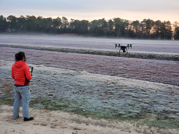
Fig. 4 – Ryan Wicks pilots a Matrice 210 with a Zenmuse XT2 payload to collect LWIR imagery of State Bog on 03 April 2022. The flight was completed before direct sunlight hit the bog surface. You may note that there is a mist hanging low over the bog that may have effected the temperature measurements.
Future Projects
In the coming years teams at the Cranberry Station in partnership with cranberry farmers are planning to explore ways to implement drones in precision agriculture: the use of drones for scouting or fertilizer or pesticide applications at specific locations. Oiva Hannula & Sons cranberry growers have already purchased a P-40X from Leading Edge Aerial Technologies (https://leaaerialtech.com/precisionvision-40x) and have started to test ways to integrate it into their workflow for precision fertilizer or pesticide application. This drone has RTK-enable GNSS navigation to achieve higher accuracy for applying its payload at a specific target site. This is an example of a technology that benefits substantially from having accuracy of data products within a few centimeters; in order to know where to send the drone to be most accurate in its application of pesticide of fertilizer, the locations of pests or unhealthy vegetation need to be surveyed accurately. Thus the use of GCPs is extremely helpful. More recent scouting drones with multispectral images can have RTK GNSS modules installed to achieve improved accuracy on their own with out GCPs, but it is still fairly simply to survey and leave 3-4 markers deployed for years in a given field to verify or slightly improve the accuracy of data products derived form RTK-enabled drones, as well as to serve as a backup should the RTK-enhanced accuracy fail during a particular flight.
Applicator and scouting drones probably won’t ever be a panacea that works as a solution to the multitude of problems and challenges that famers face as they seek to ensure a healthy crop year after year, but they do seem to be an effective new tool that can be helpful in addressing a variety of those challenges. There are other application areas that could have talked about here, but I wanted to just give a brief overview of a few of them. There may be more articles that we publish on these or ancillary topics in the coming months and years to share updates and insights.
More Information
The images and files presented in this article can be found and downloaded from this google drive folder: https://drive.google.com/open?id=19Ivv9fJsujGujYGvOLkElg2Cab4E8LYC&usp=drive_fs
Acknowledgements
Thanks and credit to contributing authors:
UMass Agricultural Learning Center
- Jason Roach
- Vincent von Dosky
- Caleb Zimmerman
- Jake Butler
- Peter Crump
- Timothy Fistori
Lettuce Project
- Dr. Omidreza Zandvakili
Cranberry Bog LWIR Surveys
- Dr. Giverson Mupambi
- Zaw Win Naung
- Joshua (Blake) Smith