You might be wondering: does anyone love anything as much as I love MatLab? I get it, another MatLab article… Well, this one is pretty cool. Handling media files in MatLab is, not only extremely useful, but is also rewarding. To the programming enthusiast, it can be hard to learn about data structures and search algorithms and have only the facilities to apply this knowledge to text documents and large arrays of numbers. Learning about how to handle media files allows to you see how computation effects pictures, and hear how it effects music. Paired with some of the knowledge for my last two articles, one can begin to see how a variety of media-processing tools can be created using MatLab.
Audio
Audio is, perhaps, the simplest place to start. MathWorks provides two built-in functions for handling audio: audioread() & audiowrite(). As the names may suggest, audioread can read-in an audio file from your machine and turn it into a matrix; audiowrite can take a matrix and write it to your computer as a new audio file. Both functions can tolerate most conventional audio file formats (WAV, FLAC, M4A, etc…); however, there is an asymmetry between the two function in that, while audioread can read-in MP3 files, audiowrite cannot write MP3 files. Still, there are a number of good, free MP3 encoders out there that can turn your WAV or FLAC file into an MP3 after you’ve created it.
So let’s get into some details… audioread has only one input argument (actually, it can be used with more than one, but for our purposed, you only have to use one), the filename. Please note, filename here means the directory too (:C\TheDirectory\TheFile.wav). If you want to select the file off your computer, you could use uigetfile for this.
The audioread function has two output arguments: the matrix of samples from the audio file & the sample rate. I would encourage the reader to save both since the sample rate will prove to be important in basically every useful process you could perform on the audio. Sample values in the audio matrix are represented by doubles and are normalized (the maximum value is 1).
Once you have the audio file read-in to MatLab, you can do a whole host of things to it. MatLab has in-built filtering and other digital signal processing tools that you can use to modify the audio. You can also make plots of the audio magnitude as well as it’s frequency contents using the fft() function. The plot shown below is of the frequency content of All Star by Smashmouth.Once you’re finished processing the audio, you can write it back to a file on your computer. This is done using the audiowrite() function. The input arguments to audiowrite are the filename, audio matrix in Matlab, and sample rate. Once again, the filename should also include the directory you want to save in. This time, the filename should also include the file extension (.wav, .ogg, .flac, .m4a, .mp4). With only this information, MatLab will produce a usable audio file that can then be played through any of your standard media players.
The audiowrite function also allows for some more parameters to be specified when creating your audiofile. Name-argument pairs can be sent as arguments to the function (after the filename, matrix, and sample-rate) and can be used to set a number of different parameters. For example, ‘BitsPerSample’ allows you to specify the bit-depth of the output file (the default is 16 bits, the standard for audio CDs). ‘BitRate’ allows you to specify the amount of compression if you’re creating an .m4a or .mp4 file. You can also use these arguments to put in song titles and artist names for use with software like iTunes.
Images
Yes, MatLab can also do pictures. There are two functions associated with handling images: imread() and imwrite(). I think you can surmise from the names of these two function which one reads-in images and which one writes them out. With images, samples exist in space rather than in time so there is no sample-rate to worry about. Images still do have a bit-depth and, in my own experience, it tends to differ a lot more from image-to-image than it does for audio files.
When you import an image into MatLab, the image is represented by a three-dimensional matrix. For each color channel (red, green, and blue), there is a two-dimensional matrix with the same vertical and horizontal resolution as your photo. When you display the image, the three channels are summed together to produce a full-color image.
By the way, if you want to display an image in MatLab, use the image() function.
MathWorks provides a good deal of image-processing features built-into MatLab so if you are interested in doing some crazy stuff to your pictures, you’re covered!
Hey wow, look at this! I’ve finally rallied myself to write a blog article about something that is not digital audio! Don’t get too excited though, this is still going to be a MATLAB article and, although I am not going to be getting too deep into any DSP, the fundamental techniques underlined in this article can be applied to a wide range of problems.
Now, let me go on record here and say I am not much of a computer programmer. Thus, if you are looking for a guide to functional programming in general, this is not the place for you! However, if you are perhaps an engineering student who’s learned MATLAB for school and are maybe interested in learning what this language is capable of, this is a good place to start. Alternatively, if you are familiar with functional languages (*cough cough* Python), then this article may help you to start transposing your knowledge to a new language.
So What are Functions?
I am sure that, depending on who you ask, there are a lot of definitions for what a function actually is. Functions in MATLAB more or less follow the standard signals-and-systems model of a system; this is to say they have a set of inputs and a corresponding set of outputs. There we go, article finished, we did it!
Joking aside, there is not much more to be said about how functions are used in MATLAB; they are excellently simple. Functions in MATLAB do provide great flexibility though because they can have as many inputs and outputs as you choose (and the number of inputs does not have to be the same as the number of outputs) and the relationship between the inputs and outputs can be whatever you want it to be. Thus, while you can make a function that is a single-input-single-output linear-time-invariant system, you can also make literally anything else.
How to Create and Use Functions
Before you can think about functions, you’ll need a MATLAB script in which to call your function(s). If you are familiar with an object oriented language (*cough cough* Java), the script is similar to your main method. Below, I have included a simple script where we create two numbers and send them to a function called noahFactorial.
Simple Script Example
It doesn’t really matter what noahFactorial does, the only thing that matters here is that the function has two inputs (here X and Y) and one output (Z).
Our actual call to the noahFactorial function happens on line 4. On the same line, we also assign the output of noahFactorial to the variable Z. Line 6 has a print statement that will print the inputs and outputs to the console along with some text.
Now looking at noahFactorial, we can see how we define and write a function. We start by writing ‘function’ and then defining the function output. Here, the output is just a single variable, but if we were to change ‘output’ to ‘[output1, output2]’, our function would return a 2×1 array containing two output values.
Simple Function Example
Some of you more seasoned programmers might notice that ‘output’ is not given a datatype. This will undoubtedly make some of you feel uncomfortable but I promise it’s okay; MATLAB is pretty good at knowing what datatype something should be. One benefit of this more laissez-faire syntax is that ‘output’ itself doesn’t even have to be a single variable. If you can keep track of it, you can make ‘output’ a 2×1 array and treat the two values like two separate outputs.
Once we write our output, we put an equals sign down (as you might expect), write the name of our function, and put (in parentheses) the input(s) to our function. Once again, the typing on the inputs is pretty soft so those too can be arrays or single values.
In all, a function declaration should look like:
function output = functionName(input)
or…
function [output1, output2, …, outputN] = functionName(input1, input2, …,inputM)
And just to reiterate, N and M here do not have to be the same.
Once inside our function, we can do whatever MATLAB is capable of. Unlike Java, return statements are not used to send anything to the output, rather they are used to stop the function in its tracks. Usually, I will assign an output for error messages; if something goes wrong, I will assign a value to the error output and follow that with ‘return’. Doing this sends back the error message and stops the function at the return statement.
So, if we don’t use return statements, then how do we send values to the output? We make sure that in our function, we have variables with the same name as the outputs. We assign those variable values in the function. On the last line of the function when the function ends, whatever the values are in the output variables, those values are sent to the output.
For example, if we define an output called X and somewhere in our function we write ‘X=5;’ and we don’t change the value of X before the function ends, the output X will have the value: 5. If we do the same thing but make another line of code later in the function that says ‘X=6;’, then the value of X returned will be: 6. Nice and easy.
…And it’s that simple. The thing I really love about functions is that they do not have to be associated with a script or with an object, you can just whip one up and use it. Furthermore, if you find you need to perform some mathematical operation often, write one function and use it with as many different scripts as you want! This insane flexibility allows for some insane problem-solving capability.
Once you get the hang of this, you can do all sorts of things. Usually, when I write a program in MATLAB, I have my main script (sometimes a .fig file if I’m writing a GUI) in one folder, maybe with some assorted text and .csv files, and a whole other folder full of functions for all sorts of different things. The ability to create functions and some good programming methodology can allow even the most novice of computer programmers to create incredibly useful programs in MATLAB.
NOTE:For this article, I used Sublime Text to write-out the examples. If you have never used MATLAB before and you turn it on for the first time and it looks completely different, don’t be alarmed! MATLAB comes pre-packaged with its own editor which is quite good, but you can also write MATLAB code in another editor, save it as a .m file, and then open it in the MATLAB editor or run it though the MATLAB kernel later.
Digital audio again? Ah yes… only in this article, I will set out to examine a simple yet complicated question: how does the sampling rate of digital audio affect its quality? If you have no clue what the sampling rate is, stay tuned and I will explain. If you know what sampling rate is and want to know more about it, also stay tuned; this article will go over more than just the basics. If you own a recording studio and insist on recording every second of audio in the highest possible sampling rate to get the best quality, read on and I hope inform you of the mathematical benefits of doing so…
What is the Sampling Rate?
In order for your computer to be able to process, store, and play back audio, the audio must be in a discrete-time form. What does this mean? It means that, rather than the audio being stored as a continuous sound-wave (as we hear it), the sound-wave is broken up into a bunch of infinitesimally small points. This way, the discrete-time audio can be represented as a list of numerical values in the computer’s memory. This is all well and good but some work needs to be done to turn a continuous-time (CT) sound-wave into a discrete-time (DT) audio file; that work is called sampling.
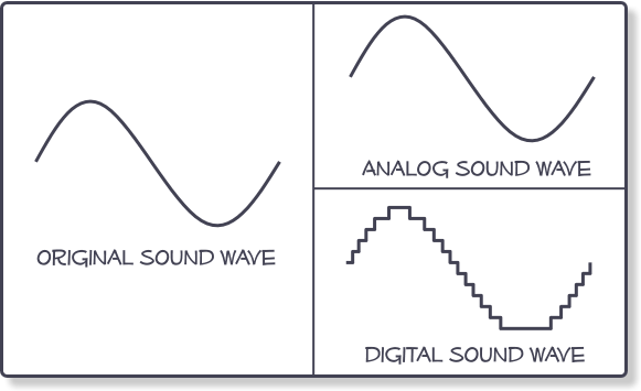
Sampling is the process of observing and recording the value of a complex signal during uniform intervals of time. Figure 1(a) is ‘analog’ sampling where this recorded value is not modified by the sampling process and figure 1(b) is digital sampling where the recorded value is quarantined so it can be represented with a binary word.
During sampling, the amplitude (loudness) of the CT wave is measured and recorded at regular intervals to create the list of values that make up the DT audio file. The inverse of this sampling interval is known as the sample rate and has a unit of Hertz (Hz). By far, the most common sample rate for digital audio is 44100 Hz; this means that the CT sound-wave is sampled 44100 times every second.
This is a staggering number of data points! On a audio CD, each sample is represented by two bytes; that means that one second of audio will take up over 170 KB of space! Why is all this necessary? you may ask…
The Nyquist-Shannon Sampling Theorem
Some of you more interested readers may have heard already of the Nyquist-Shannon Sampling Theorem (some of you may also know this theorem simply as the Nyquist Theorem). The Nyquist-Shannon Theorem asserts that any CT signal can be sampled, turned into a DT file, and then converted back into a CT signal with no loss in information so long as one condition is met: the CT signal is band-limited at the Nyquist Frequency. Let’s unpack this…
Firstly, what does it mean for a signal to be band-limited? Every complex sound-wave is made up of a whole myriad of different frequencies. To illustrate this point, below is the frequency spectrum (the graph of all the frequencies in a signal) of All Star by Smash Mouth:
Smash Mouth is band-limited! How do we know? Because the plot of frequencies ends. This is what it means for a signal to be band-limited: it does not contain any frequencies beyond a certain point. Human hearing is band-limited too; most humans cannot hear any frequencies above 20,000 Hz!
So, I suppose then we can take this to mean that, if the Nyquist frequency is just right, any audible sound can be represented in digital form with no loss in information? By this theorem, yes! Now, you may ask, what does does the Nyquist frequency have to be for this to happen?
For the Shannon-Nyquist Sampling Theorem to hold, the Nyquist frequency must be greater than twice the highest frequency being sampled. For sound, the highest frequency is 20 kHz; and thus, the Nyquist frequency required for sampled audio to capture sound with no loss in information is… 40 kHz. What was that sample-rate I mentioned earlier? You know, that one that is so common that basically all digital audio uses it? It was 44.1 kHz. Huzzah! Basically all digital audio is a perfect representation of the original sound it is representing! Well…
Aliasing: the Nyquist Theorem’s Complicated Side-Effect
Just because we cannot hear sound about 20 kHz does not mean it does not exist; there are plenty of sound-waves at frequencies higher than humans can hear.
So what happens to these higher sound-waves when they are sampled? Do they just not get recorded? Unfortunately no…
A visual illustration of how under-sampling a frequency results in some unusual side-effects. This unique kind of error is known as ‘aliasing’
So if these higher frequencies do get recorded but frequencies above the Nyquist frequency cannot be sampled correctly, then what happens to them? They are falsely interprated as lower frequencies and superimposed over the correctly sampled frequencies. The distance between the high frequency and the Nyquist frequency govern what lower frequency these high-frequency signals will be interpreted as. To illustrate this point, here is an extreme example…
Say we are trying to sample a signal that contains two frequencies: 1 Hz and 3 Hz. Due to poor planning, the Nyquist frequency is selected to be 2 Hz (meaning we are sampling at a rate of 4 Hz). Further complicating things, the 3 Hz cosine-wave is offset by 180° (meaning the waveform is essentially multiplied by -1). So we have the following two waveforms….
When the two waves are superimposed to create one complicated waveform, it looks like this…
Superimposed waveform constructed from the 1 Hz and 3 Hz waves
Pretty, right? Well unfortunately, if we try to sample this complicated waveform at 4 Hz, do you know what we get? Nothing! Zero! Zilch! Why is this? Because when the 3 Hz cosine wave is sampled and reconstructed, it is falsely interpreted as a 1 Hz wave! Its frequency is reflected about the Nyquist frequency of 2 Hz. Since the original 1 Hz wave is below the Nyquist frequency, it is interpreted with the correct frequency. So we have two 1 Hz waves but one of them starts at 1 and the other at -1; when they are added together, they create zero!
Another way we can see this phenomena is by looking at the graph. Since we are sampling at 4 Hz, that means we are observing and recording four evenly-spaced points between zero and one, one and two, three and four, etc… Take a look at the above graph and try to find 4 evenly-space points between zero and one (but not including one). You will find that every single one of these points corresponds with a value of zero! Wow!
So aliasing can be a big issue! However, designers of digital audio recording and processing systems are aware of this and actually provision special filters (called anti-aliasing filters) to get rid of these unwanted effects.
So is That It?
Nope! These filters are good, but they’re not perfect. Analog filters cannot just chop-off all frequencies above a certain point, they have to, more or less, gradually attenuate them. So this means designers have a choice: either leave some high frequencies and risk distortion from aliasing or roll-off audible frequencies before they’re even recorded.
And then there’s noise… Noise is everywhere, all the time, and it never goes away. Modern electronics are rather good at reducing the amount of noise in a signal but they are far from perfect. Furthermore noise tends to be mostly present at higher frequencies; exactly the frequencies that end up getting aliased…
What effect would this have on the recorded signal? Well if we believe that random signal noise is present at all frequencies (above and below the Nyquist frequency), then our original signal would be masked with a layer of infinitely-loud aliased noise. Fortunately for digitally recorded music, the noise does stop at very high frequencies due to transmission-line effects (a much more complicated topic).
What can be Learned from All of This?
The end result of this analysis on sample rate is that the sample rate alone does not tell the whole story about what’s being recorded. Although 44.1 kHz (the standard sample rate for CDs and MP3 files) may be able to record frequencies up to 22 kHz, in practice a signal being sampled at 44.1 kHz will have distortion in the higher frequencies due to high frequency noise beyond the Nyquist frequency.
So then, what can be said about recording at higher sample rates? Some new analog-to-digital converts for musical recording sample at 192 kHz. Most, if not all, of the audio recording I do is done at a sample rate of 96 kHz. The benefit to recording at the higher sample rates is that you can recording high-frequency noise without it causing aliasing and distortion in the audible range. With 96 kHz, you get a full 28 kHz of bandwidth beyond the audible range where noise can exist without causing problems. Since signals with frequencies up to around 9.8 MHz can exist in a 10 foot cable before transmission line effects kick in, this is extremely important!
And with that, a final correlation can be predicted: the greater the sample rate, the less noise will result in aliasing in the audible spectrum. To those of you out there who have insisted that the higher sample rates sound better, maybe now you’ll have some heavy-duty math to back up your claims!
Since the dawn of digital computation, the machine has only known one language: binary. This strange concoction of language and math has existed physically in many forms since the beginning. In its simplest form, binary represents numerical values using only two values, 1 and 0. This makes mathematical operations very easy to perform with switches. It also makes it very easy to store information in a very compact manor.
Early iterations of data storage employed some very creative thinking and some strange properties of materials.
IBM 80-Column Punch Card
One of the older (and simpler) methods of storing computer information was on punch cards. As the name suggests, punch cards would have sections punched out to indicate different values. Punch cards allowed for the storage of binary as well as decimal and character values. However, punch cards had an extremely low capacity, occupied a lot of space, and were subject to rapid degradation. For these reasons, punch cards became phased out along with black and white TV and drive-in movie theaters.
Macroscopic Image of Ferrite Memory Cores
Digital machines had the potential to view and store data using far less intuitive methods. King of digital memory from the 1960s unto the mid-to-late 70s was magnetic core memory. By far one of the prettiest things ever made for the computer, this form of memory was constructed with a lattice of interconnected ferrite beads. These beads could be magnetized momentarily when a current of electricity passed near them. Upon demagnetizing, they would induce a current in nearby wire. This current could be used to measure the binary value stored in that bead. Current flowing = 1, no current = 0.
Even more peculiar was the delay-line memory used in the 1960s. Though occasionally implemented on a large scale, the delay-line units were primarily used from smaller computers as there is no way they were even remotely reliable… Data was stored in the form of pulsing twists through a long coil of wire. This mean that data could be corrupted if one of your fellow computer scientists slammed the door to the laboratory or dropped his pocket protector near the computer or something. This also meant that the data in the coil had to be constantly read and refreshed every time the twists traveled all the way through the coil which, as anyone who has ever played with a spring before knows, does not take a long time.
Delay-Line Memory from the 1960s
This issue of constant refreshing may seem like an issue of days past, but DDR memory, the kind that is used in modern computers, also has to do this. The DDR actually stands for double data rate and refers to the number of times every cycle that the data in every binary cell is copied into an adjacent cell and then copied back. This reduces the amount of useful work per clock cycle that a DDR memory unit can do. Furthermore, only 64 bits of the 72-bit DIMM connection used for DDR memory are actually used for data (the rest are for Hamming error correction). So we only use about half the work that DDR memory does for actual computation and it’s still so unreliable that we need a whole 8 bits for error correction; perhaps this explains why most computers now come with three levels of cache memory whose sole purpose is to guess what data the processor will need in the hopes that it will reduce the processor’s need to access the RAM.
DDR Memory Chip on a Modern RAM Stick
Even SRAM (the faster and more stable kind of memory used in cache) is not perfect and it is extremely expensive. A MB of data on a RAM stick will run you about one cent while a MB of cache can be as costly as $10. What if there were a better way or making memory that was more similar to those ferrite cores I mentioned earlier? What if this new form of memory could also be written and read to with speeds orders of magnitude greater than DDR RAM or SRAM cache? What if this new memory also shared characteristics with human memory and neurons?
Enter: Memristors and Resistive Memory
As silicon-based transistor technology looks to be slowing down, there is something new on the horizon: resistive RAM. The idea is simple: there are materials out there whose electrical properties can be changed by having a voltage applied to them. When the voltage is taken away, these materials are changed and that change can be measured. Here’s the important part: when an equal but opposite voltage is applied, the change is reversed and that reversal can also be measured. Sounds like something we learned about earlier…
The change that takes place in these magic materials is in their resistivity. After the voltage is applied, the extent to which these materials resist a current of electricity changes. This change can be measured and therefor binary data can be stored.
A Microscopic Image of a Series of Memristors
Also at play in the coming resistive memory revolution is speed. Every transistor ever made is subject to something called propagation delay: the amount of time required for a signal to traverse the transistor. As transistors get smaller and smaller, this time is reduced. However, transistors cannot get very much smaller because of quantum uncertainty in position: a switch is no use if the thing you are trying to switch on and off can just teleport past the switch. This is the kind of behavior common among very small transistors.
Because the memristor does not use any kind of transistor, we could see near-speed-or-light propagation delays. This means resistive RAM could be faster than DDR RAM, faster than cache, and someday maybe even faster than the registers inside the CPU.
There is one more interesting aspect here. Memristors also have a tendency to “remember” data long after is has been erased and over written. Now, modern memory also does this but, because the resistance of the memristor is changing, large arrays of memristors could develop sections with lower resistance due to frequent accessing and overwriting. This behavior is very similar to the human brain; memory that’s accessed a lot tends to be easy to… well… remember.
Resistive RAM looks to be, at the very least, a part of the far-reaching future of computing. One day we might have computers which can not only recall information with near-zero latency, but possibly even know the information we’re looking for before we request it.
When I left New York in January, the city was in high spirits about its extensive Subway System. After almost 50 years of construction, and almost 100 years of planning, the shiny, new Second Avenue subway line had finally been completed, bringing direct subway access to one of the few remaining underserved areas in Manhattan. The city rallied around the achievement. I myself stood with fellow elated riders as the first Q train pulled out of the 96th Street station for the first time; Governor Andrew Cuomo’s voice crackling over the train’a PA system assuring riders that he was not driving the train.
In a rather ironic twist of fate, the brand-new line was plagued, on its first ever trip, with an issue that has been effecting the entire subway system since its inception: the ever present subway delay.
A small group of transit workers gathered in the tunnel in front of the stalled train to investigate a stubborn signal. The signal was seeing its first ever train, yet its red light seemed as though it had been petrified by 100 years of 24-hour operation, just like the rest of them.
Track workers examine malfunctioning signal on Second Avenue Line
When I returned to New York to participate in a summer internship at an engineering firm near Wall Street, the subway seemed to be falling apart. Having lived in the city for almost 20 years and having dealt with the frequent subway delays on my daily commute to high school, I had no reason to believe my commute to work would be any better… or any worse. However, I started to see things that I had never seen: stations at rush hour with no arriving trains queued on the station’s countdown clock, trains so packed in every car that not a single person was able to board, and new conductors whose sole purpose was to signal to the train engineers when it was safe to close the train doors since platforms had become too consistently crowded to reliably see down.
At first, I was convinced I was imagining all of this. I had been living in the wide-open and sparsely populated suburbs of Massachusetts and maybe I had simply forgotten the hustle and bustle of the city. After all, the daily ridership on the New York subway is roughly double the entire population of Massachusetts. However, I soon learned that the New York Times had been cataloging the recent and rapid decline of the city’s subway. In February, the Times reported a massive jump in the number of train delays per month, from 28,000 per month in 2012 up to 70,000 at the time of publication.
What on earth had happened? Some New Yorkers have been quick to blame Mayor Bill De’Blasio However, the Metropolitan Transportation Authority, the entity which owns and operates the city subway, is controlled by the state and thus falls under the jurisdiction of Governor Andrew Cuomo. However, it’s not really Mr. Cuomo’s fault either. In fact, it’s no one person’s fault at all! The subway has been dealt a dangerous cocktail of severe overcrowding and rapidly aging infrastructure.
Thinking Gears that Run the Trains
Anyone with an interest in early computer technology is undoubtedly familiar with the mechanical computer. Before Claude Shannon invented electronic circuitry that could process information in binary, all we had to process information were large arrays of gears, springs, and some primitive analog circuits which were finely tuned to complete very specific tasks. Some smaller mechanical computers could be found aboard fighter jets to help pilots compute projectile trajectories. If you saw The Imitation Game last year, you may recall the large computer Alan Turing built to decode encrypted radio transmissions during the Second World War.
Interlocking machine similar to that used in the NYC subway
New York’s subway had one of these big, mechanical monsters after the turn of the century; In fact, New York still has it. Its name is the interlocking machine and it’s job is simple: make sure two subway trains never end up in the same place at the same time. Yes, this big, bombastic hunk of metal is all that stands between the train dispatchers and utter chaos. Its worn metal handles are connected directly to signals, track switches, and little levers designed to trip the emergency breaks of trains that roll past red lights.
The logic followed by the interlocking machine is about as complex as engineers could make it in 1904:
Sections of track are divided into blocks, each with a signal and emergency break-trip at their entrance.
When a train enters a block, a mechanical switch is triggered and the interlocking machine switches the signal at the entrance of the block to red and activates the break-trip.
After the train leaves the block, the interlocking machine switches the track signal back to green and deactivates the break-trip.
Essentially a very large finite-state machine, this interlocking machine was revolutionary back at the turn of the century. At the turn of the century, however, some things were also acting in the machine’s favor; for instance, there were only three and a half million people living in New York at the time, they were all only five feet tall, and the machine was brand new.
As time moved on, the machine aged and so did too did the society around it. After the Second World War, we replaced the bumbling network of railroads with an even more extensive network of interstate highways. The train signal block, occupied by only one train at a time, was replaced by a simpler mechanism: the speed limit.
However, the MTA and the New York subways have lagged behind. The speed and frequency of train service remains limited by how many train blocks were physically built into the interlocking machines (yes, in full disclosure, there is more than one interlocking machine but they all share the same principles of operation). This has made it extraordinarily difficult for the MTA to improve train service; all the MTA can do is maintain the again infrastructure. The closest thing the MTA has to a system-wide software update is a lot of WD40.
Full-Steam Ahead
There is an exception to the constant swath of delays…two actually. In the 1990s and then again recently, the MTA did yank the old signals and interlocking machines from two subway lines and replace them with a fully automated fleet of trains, controlled remotely by a digital computer. In a odd twist of fate, the subway evolved straight from its Nineteenth Century roots straight to Elon Musk’s age of self-driving vehicles.
The two lines selected were easy targets, both serve large swaths of suburb in Brooklyn and Queens and both are two-track lines, meaning they have no express service. This made the switch to automated trains easy and very effective for moving large numbers of New Yorkers. And the switch was effective! Of all the lines in New York, the two automated lines have seen the least reduction in on-time train service. The big switch also had some more proactive benefits, like the addition of accurate countdown clocks in stations, a smoother train ride (especially when stopping and taking off), and the ability for train engineers to play Angry Birds during their shifts (yes, I have seen this).
The first to receive the update was the city’s, then obscure, L line. The L is one of the only two trains to traverse the width of the Manhattan Island and is the transportation backbone for many popular neighborhoods in Brooklyn. In recent years, these neighborhoods have seen a spike in population due, in part, to frequent and reliable train service.
L train at its terminal station in Canarsie, Brooklyn
The contrast between the automated lines and the gear-box-controlled lines is astounding. A patron of the subway can stand on a train platform waiting for an A or C train for half an hour… or they could stand on another platform and see two L trains at once on the same stretch of track.
The C line runs the oldest trains in the system, most of them over 50 years old.
The city also elected to upgrade the 7 line; the only other line in the city to traverse the width of Manhattan and one of only two main lines to run through the center of Queens. Work on the 7 is set to finish soon and the results looks to be promising.
Unfortunately for the rest of the city’s system, the switch to automatic train control for those two lines was not cheap and it was not quick. In 2005, it was estimated that a system-wide transition to computer controlled trains would not be completed until 2045. Some other cities, most notably London, made the switch to automated trains years ago. It is though to say why New York has lagged behind, but it most likely has to do with the immense ridership of the New York system.
New York is the largest American city by population and by land area. This makes other forms of transportation far less viable when traveling though the city. After a the public opinion of highways in the city was ruined in the 1960s following the destruction of large swaths of the South Bronx, many of the city’s neighborhoods have been left nearly inaccessible via car. Although New York is a very walkable city, its massive size makes commuting by foot from the suburbs to Manhattan impractical as well. Thus the subways must run every day and for every hour of the day. If the city wants to shut down a line to do repairs, they often cant. Often times, line are only closed for repairs on weekends and nights for a few hours.
Worth the Wait?
Even though it may take years for the subway to upgrade its signals, the city has no other option. As discussed earlier, the interlocking machine can only support so many trains on a given length of track. On the automated lines, transponders are placed every 500 feet, supporting many more trains on the same length of track. Trains can also be stopped instantly instead of having to travel to the next red-signaled block. With the number of derailments and stalled trains climbing, this unique ability of the remote-controlled trains is invaluable. Additionally, automated trains running on four-track lines with express service could re-route instantly to adjacent tracks in order to completely bypass stalled trains. Optimization algorithms could be implemented to have a constant and dynamic flow of trains. Trains could be controlled more precisely during acceleration and breaking to conserve power and prolong the life of the train.
For the average New Yorker, these changes would mean shorter wait times, less frequent train delays, and a smoother and more pleasant ride. In the long term, the MTA would most likely save millions of dollars in repair costs without the clunky interlocking machine. New Yorkers would also save entire lifetimes worth of time on their commutes. The cost may be high, but unless the antiquated interlocking machines are put to rest, New York will be paying for it every day.
Since the dawn of time, humans have been attempting to record music. For the vast majority of human history, this has been really really difficult. Early cracks at getting music out of the hands of the musician involved mechanically triggered pianos whose instructions for what to play were imprinted onto long scrolls of paper. These player pianos were difficult to manufacture (this was prior to the industrial revolution) and not really viable for casual music listening. There was also the all-important phonograph, which recorded sound itself mechanically onto the surface of a wax cylinder.
If it sounds like the aforementioned techniques were difficult to use and manipulate, it was! Hardly anyone owned a phonograph since they were expensive, recordings were hard to come by, and they really didn’t sound all that great. Without microphones or any kind of amplification, bits of dust and debris which ended up on these phonograph records could completely obscure the original recording behind a wall of noise.
Humanity had a short stint with recording sound as electromagnetic impulses on magnetic tape. This proved to be one of the best ways to reproduce sound (and do some other cool and important things too). Tape was easy to manufacture, came in all different shapes and sizes, and offered a whole universe of flexibility for how sound could be recorded onto it. Since tape recorded an electrical signal, carefully crafted microphones could be used to capture sounds with impeccable detail and loudspeakers could be used to play back the recorded sound at considerable volumes. Also at play were some techniques engineers developed to reduce the amount of noise recorded onto tape, allowing the music to be front and center atop a thin floor of noise humming away in the background. Finally, tape offered the ability to record multiple different sounds side-by-side and play them back at the same time. These side-by-side sounds came to be known as ‘tracks’ and allowed for stereophonic sound reproduction.
Tape was not without its problems though. Cheap tape would distort and sound poor. Additionally, tape would deteriorate over time and fall apart, leaving many original recordings completely unlistenable. Shining bright on the horizon in the late 1970s was digital recording. This new format allowed for low-noise, low cost, and long-lasting recordings. The first pop music record to be recorded digitally was Ry Cooder’s, Bop till you Drop in 1979. Digital had a crisp and clean sound that was rivaled only by the best of tape recording. Digital also allowed for near-zero degradation of sound quality once something was recorded.
Fast-forward to today. After 38 years of Moore’s law, digital recording has become cheap and simple. Small audio recorders are available at low cost with hours and hours of storage for recording. Also available are more hefty audio interfaces which offer studio-quality sound recording and reproduction to any home recording enthusiast.
Basic Components: What you Need
Depending on what you are trying to record, your needs may vary from the standard recording setup. For most users interested in laying down some tracks, you will need the following.
Audio Interface (and Preamplifier): this component is arguably the most important as it connects everything together. The audio interface contains both analog-to-digital converters and a digital-to-analog convert; these allow it to both turn sound into the language of your computer for recording, and turn the language of your computer back into sound for playback. These magical little boxes come in many shapes and sizes; I will discus these in a later section, just be patient.
Digital Audio Workstation (DAW) Software: this software will allow your computer to communicate with the audio interface. Depending on what operating system you have running on your computer, there may be hundreds of DAW software packages available. DAWs vary greatly in complexity, usability, and special features; all will allow you the basic feature of recording digital audio from an audio interface.
Microphone: perhaps the most obvious element of a recording setup, the microphone is one of the most exciting choices you can make when setting up a recording rig. Microphones, like interfaces and DAWs, come in all shapes a sizes. Depending on what sound you are looking for, some microphones may be more useful than others. We will delve into this momentarily.
Monitors (and Amplifier): once you have set everything up, you will need a way to hear what you are recording. Monitors allow you to do this. In theory, you can use any speaker or headphone as a monitor. However, some speakers and headphones offer more faithful reproduction of sound without excessive bass and can be better for hearing the detail in your sound.
Audio Interface: the Art of Conversion
Two channel USB audio interface.
The audio interface can be one of the most intimidating elements of recording. The interface contains the circuitry to amplify the signal from a microphone or instrument, convert that signal into digital information, and then convert that information back to an analog sound signal for listening on headphones or monitors.
Interfaces come in many shapes and sizes but all do similar work. These days, most interfaces offer multiple channels of recording at one time and can record in uncompressed CD-audio quality or better.
Once you step into the realm of digital audio recording, you may be surprised to find a lack of mp3 files. Turns out, mp3 is a very special kind of digital audio format and cannot be recorded to directly; mp3 can only be created from existing audio files in non-compressed formats.
You may be asking yourself, what does it mean for audio to be compressed? As an electrical engineer, it may be hard for me to explain this in a way that humans can understand, but I will try my best. Audio takes up a lot of space. Your average iPhone or Android device maybe has 32 GB of space but most people can keep thousands of songs on their device. This is done using compression. Compression is the computer’s way of listening to a piece of music, and removing all the bits and pieces that most people wont notice. Soft and infrequent noises, like the sound of a guitarist’s fingers scraping a string, are removed while louder sounds, like the sound of the guitar, are left in. This is done using the Fourier Transform and a bunch of complicated mathematical algorithms that I don’t expect anyone reading this to care about.
When audio is uncompressed, a few things are true: it takes up a lot of space, it is easy to manipulate with digital effects, and it often sounds very, very good. Examples of uncompressed audio formats are: .wav on Windows, .aif and .aiff on Macintosh, and .flac for all the free people of the Internet. Uncompressed audio comes in many different forms but all have two numbers which describe their sound quality: ‘word length’ or ‘bit depth’ and ‘sample rate.’
The information for digital audio is contained in a bunch of numbers which indicate the loudness or volume of the sound at a specific time. The sample rate tells you how many times per second the loudness value is captured. This number needs to be at least two times higher than the highest audible frequency, otherwise the computer will perceive high frequencies as being lower than they actually are. This is because of the Shannon Nyquist Theorem which I, again, don’t expect most of you to want to read about. Most audio is captured at 44.1 kHz, making the highest frequency it can capture 22.05 kHz, which is comfortably above the limits of human hearing.
The word length tells you how many numbers can be used to represent different volumes of loudness. The number of different values for loudness can be up to 2^word length. CDs represent audio with a word length of 16 bits, allowing for 65536 different values for loudness. Most audio interfaces are capable of recording audio with a 24-bit word length, allowing for exquisite detail. There are some newer systems which allow for recording with a 32-bit word length but these are, for the majority part, not available at low-cost to consumers.
I would like to add a quick word about USB. There is a stigma, in the business, against USB audio interfaces. Many interfaces employ connectors with higher bandwidth, like FireWire and Thunderbolt, and charge a premium for it. It may seem logical, faster connection, better quality audio. Hear this now: no audio interface will ever be sold which has a connector that is too slow for the quality audio it can record. This is to say, USB can handle 24-bit audio with a 96 kHz sample rate, no problem. If you notice latency in your system, it is from the digital-to-analog and analog-to-digital converters as well as the speed of your computer; latency in your recording setup has nothing to do with what connector your interface uses. It may seem like I am beating a dead horse here, but many people think this and it’s completely false.
One last thing before we move on to the DAW, I mentioned earlier that frequencies above half the recording sample rate will be perceived, by your computer, as lower frequencies. These lower frequencies can show up in your recording and can cause distortion. This phenomena has a name and it’s called aliasing. Aliasing doesn’t just happen with audible frequencies, it can happen with super-sonic sound too. For this reason, it is often advantageous to record at higher sample rates to avoid having these higher frequencies perceived within the audible range. Most audio interfaces allow for recording 24-bit audio with a 96 kHz sample rate. Unless you’re worried about taking up too much space, this format sounds excellent and offers the most flexibility and sonic detail.
Digital Audio Workstation: all Out on the Table
Apple’s pro DAW software: Logic Pro X
The digital audio workstation, or DAW for short, is perhaps the most flexible element of your home-studio. There are many many many DAW software packages out there, ranging in price and features. For those of you looking to just get into audio recording, Audacity is a great DAW to start with. This software is free and simple. It offers many built-in effects and can handle the full recording capability of any audio interface which is to say, if you record something well on this simple and free software, it will sound mighty good.
Here’s the catch with many free or lower-level DAWs like Audacity or Apple’s Garage Band: they do not allow for non-destructive editing of your audio. This is a fancy way of saying that once you make a change to your recorded audio, you might not be able to un-make it. Higher-end DAWs like Logic Pro and Pro Tools will allow you to make all the changes you want without permanently altering your audio. This allows you to play around a lot more with your sound after its recorded. More expensive DAWs also tend to come with a better-sounding set of built-in effects. This is most noticeable with more subtle effects like reverb.
There are so many DAWs out there that it is hard to pick out a best one. Personally, I like Logic Pro, but that’s just preference; many of the effects I use are compatible with different DAWs so I suppose I’m mostly just used to the user-interface. My recommendation is to shop around until something catches your eye.
The Microphone: the Perfect Listener
Studio condenser and ribbon microphones.
The microphone, for many people, is the most fun part of recording! They come in many shapes and sizes and color your sound more than any other component in your setup. Two different microphones can occupy polar opposites in the sonic spectrum.
There are two common types of microphones out there: condenser and dynamic microphones. I can get carried away with physics sometimes so I will try not to write too much about this particular topic.
Condenser microphones are a more recent invention and offer the best sound quality of any microphone. They employ a charged parallel plate capacitor to measure vibrations in the air. This a fancy way of saying that the element in the microphone which ‘hears’ the sound is extremely light and can move freely even when motivated by extremely quiet sounds.
Because of the nature of their design, condenser microphones require a small amplifier circuit built-into the microphone. Most new condenser microphones use a transistor-based circuit in their internal amplifier but older condenser mics employed internal vacuum-tube amplifiers; these tube microphones are among some of the clearest and most detailed sounding microphones ever made.
Dynamic microphones, like condenser microphones, also come in two varieties, both emerging from different eras. The ribbon microphone is the earlier of the two and observes sound with a thin metal ribbon suspended in a magnetic field. These ribbon microphones are fragile but offer a warm yet detailed quality-of-sound.
The more common vibrating-coil dynamic microphone is the most durable and is used most often for live performance. The prevalence of the vibrating-coil microphone means that the vibrating-coil is often dropped from the name (sometimes the dynamic is also dropped from the name too); when you use the term dynamic mic, most people will assume you are referring to the vibrating-coil microphone.
With the wonders of globalization, all microphones can be purchase at similar costs. Though there is usually a small premium to purchase condenser microphones over dynamic mics, costs can remain comfortably around $100-150 for studio-quality recording mics. This means you can use many brushes to paint your sonic picture. Often times, dynamic microphones are used for louder instruments like snare and bass drums, guitar amplifiers, and louder vocalists. Condenser microphones are more often used for detailed sounds like stringed instruments, cymbals, and breathier vocals.
Monitors: can You Hear It?
Studio monitors at Electrical Audio Studios, Chicago
When recording, it is important to be able to hear the sound that your system is hearing. Most people don’t think about it, but there are many kinds of monitors out there: the screen on our phones and computers which allow us to see what the computer is doing, to the viewfinder on a camera which allows us to see what the camera sees. Sound monitors are just as important.
Good monitors will reproduce sound as neutrally as possible and will only distort at very very high volumes. These two characteristics are important for monitoring as you record, and hearing things carefully as you mix. Mix?
Once you have recorded your sound, you may want to change it in your DAW. Unfortunately, the computer can’t always guess what you want your effects to sound like, so you’ll need to make changes to settings and listen. This could be as simple as changing the volume of one recorded track or it could be as complicated as correcting an offset in phase of two recorded tracks. The art of changing the sound of your recorded tracks is called mixing.
If you are using speakers as monitors, make sure they don’t have ridiculously loud bass, like most speakers do. Mixing should be done without the extra bass; otherwise, someone playing back your track on ‘normal’ speakers will be underwhelmed by a thinner sound. Sonically neutral speakers make it very easy to hear what you finished product will sound like on any system.
It’s a bit harder to do this with headphones as their proximity to your ears makes the bass more intense. I personally like mixing on headphones because the closeness to my ear allows me to hear detail better. If you are to mix with headphones, your headphones must have open-back speakers in them. This means that there is no plastic shell around the back of the headphone. With no set volume of air behind the speaker, open-back headphones can effortlessly reproduce detail, even at lower volumes.
1
Monitors aren’t just necessary for mixing, they also help to hear what you’re recording as you record it. Remember when I was talking about the number of different loudnesses you can have for 16-bit and 24-bit audio? Well, when you make a sound louder than the loudest volume you can record, you get digital distortion. Digital distortion does not sound like Jimi Hendrix, it does not sound like Metallica, it sounds abrasive and harsh. Digital distortion, unless you are creating some post-modern masterpiece, should be avoided at all costs. Monitors, as well as the volume meters in your DAW, allow you to avoid this. A good rule of thumb is: if it sounds like it’s distorting, it’s distorting. Sometimes you won’t hear the distortion in your monitors, this is where the little loudness bars on your DAW software come in; those bad boys should never hit the top.
A Quick Word about Formats before we Finish
These days, most music ends up as an mp3. Convenience is important so mp3 does have its place. Most higher-end DAWs will allow you to make mp3 files upon export. My advise to any of your learning sound-engineers out there is to just play around with formatting. However, a basic outline of some common formats may be useful…
24-bit, 96 kHz: This is best format most systems can record to. Because of large files sizes, audio in this format rarely leaves the DAW. Audio of this quality is best for editing, mixing, and converting to analog formats like tape or vinyl.
16-bit, 44.1 kHz: This is the format used for CDs. This format maintains about half of the information that you can record on most systems, but it is optimized for playback by CD players and other similar devices. Its file-size also allows for about 80 minutes of audio to fit on a typical CD. Herein lies the balance between excellent sound quality, and file-size.
mp3, 256 kb/s: Looks a bit different, right? The quality of mp3 is measured in kb/s. The higher this number, the less compressed the file is and the more space it will occupy. iTunes uses mp3 at 256 kb/s, Spotify probably uses something closer to 128 kb/s to better support streaming. You can go as high as 320 kb/s with mp3. Either way, mp3 compression is always lossy so you will never get an mp3 to sound quite as good as an uncompressed audio file.
In Conclusion
Recording audio is one of the most fun hobbies one can adopt. Like all new things, recording can be difficult when you first start out but will become more and more fulfilling over time. One can create their own orchestras at home now; a feat which would have been near impossible 20 years ago. The world has many amazing sounds and it is up to people messing around with microphone in bedrooms and closets to create more.
Form the beginning, people all around the world have shared a deep love of music. From early communication through drumming, to exceedingly complex arrangements for big bands, music has been an essential part of human communication. So it makes sense that people would push to find a way to record music as performed by the musician.
The advent of Tin-Pan Alley in New York initially produced only sheet music – the recording of music on paper, readable only by trained musicians – but it was the invention of Thomas Edison’s phonograph which altered the history of music the most. With the phonograph, sound could be recorded from the air. Early phonograph systems employed a light diaphragm, often in the shape of a horn, suspended on springs and attached to a needle which would carve into a rotating cylinder of wax. These records were made without any electric power and have a distinct sound which often wavers in tone character and pitch.
Thomas Edison with early Phonograph
In the 1920s, the RCA company developed the first electrical audio recording system which employed microphones and a magnetic medium on which to record electrical impulses. The microphone could vibrate more easily than the phonograph horn and could therefore reproduce sound in a more natural and consistent manner.
After a brief push to standardize the format for recorded music, Edison’s wax cylinder gave way to the disk-shaped Gramophone record, which eventually gave way to the two formats we are now familiar with: the 33 rpm vinyl record, for full-length albums, and the 45 rpm vinyl record, for single songs. Now obsolete, these formats allowed for exceedingly accurate reproduction of recorded sound for half a century.
Audio goes Digital
In the mid-twentieth century, Claude Shannon determined that information could be encoded into discrete values, transmitted, and decoded to reconstruct the original information. The human voice could be transmitted, not as an analog electrical representation of a sound-wave, but as a series of numbers representing the magnitude and polarity of the sound-wave at given times (samples). This method of encoding information into discrete values allowed for the more efficient use of limited resources for transmitting and storing information.
Claude Shannon: Father of Information Theory
For music, this meant that sound could be broken down into only the magnitude and polarity of the sound-wave, at a given time, and represented as a binary number. With music now a series of 1s and 0s, and with far less information encoded into these 1s and 0s than with the analog formats, music could be stored on small, plastic disks called Compact Disks. These compact disks, or CDs, contained an unadulterated digital representation of the original analog sound-wave. The CD, though sometimes thin and clinical-sounding, offered some of the most detailed reproduction of sound in history.
Digital Streaming and the Push for Compression
In the 1990s, online music sharing services birthed a new format for recorded music: the mp3. The mp3, though a digital representation of an analog sound-wave like a CD, made feasible downloading music over the internet. It did so using a simple principle: use a fourier transform to view the sound-wave as a series of sine waves of different frequencies and remove all the frequencies with low magnitudes.
Napster, an early music sharing service
While this technique allowed for digital audio files to be much smaller, it had the nasty effect of sometimes removing some important sonic character. Though insignificant sounds in a piece of music could be a small amount of background hiss, it could also be the timbre of a musical instrument. For this reason, mp3 files would often lack the fullness and detail of the CD or analog formats.
The world of Recorded Music, Post mp3
Though internet speeds have vastly improved since the early days of music streaming, compression has not gone away. The unfortunate nature of the problem is that one powerful computer can run a compression algorithm on a digital audio file in less than a second and then stream it to a user; streaming lossless digital audio, like the digital audio from a CD, requires the rebuilding of physical infrastructure to handle the extra data. From a profit-generating stance, compression is cheap and effective; most people don’t notice if audio is compressed, especially if they are listening to music on computer speakers or poorly constructed headphones.
However, there are some out there who do notice. Though services like iTunes and Spotify do not offer the purchasing of music in non-compressed formats, music in these formats can sometimes be purchased from lesser known services. CDs are also still in production and can be purchased for most new albums through services like Amazon. Some may also be surprised to learn of the prevalence of the analog formats as well; for most new releases, a new copy can be purchased on a vinyl record. Since most music is recorded directly to a digital format, vinyl records are made from digital masters. However, these masters are often of the highest quality as there is no need to conserve space on the analog formats; digital audio sampled at 44.1 kHz and 96 kHz both consume the same amount of space on the surface of a vinyl record.
So what is the answer for those looking to move beyond the realm of compressed music? Well, we could all write in to Spotify and iTunes and let them know that we will only purchase digital audio sampled at 96 kHz with a 24-bit word-length…but there may be a simpler way. CDs and vinyl records are still made and they sound great! If you have an older computer you may be able to listen to a CD without having to purchase any extra equipment. For faithful reproduction of the CD’s contents, I would recommend a media player like VLC. Additionally, if you have grandparents with an attic, you may even have the necessary equipment to play back a vinyl record. If not, the market for the analog formats seems to be getting miraculously larger as time goes on so there is more and more variety every day for phono equipment. There’s also always live music and no sound reproduction medium, no matter how accurate, can truly capture the spirit of an energetic performance.
So however you decide to listen to your music, be educated and do not settle for convenience over quality when you do not have to!
So last time we learned a few basic commands: ls, cd, and open. That will get us through about 75% of what we would normally use the Finder for, but now we are going to address the other 50% (no, those percentages are not a typo). In this article, I will address the following tasks:
-Copying and Moving
-Performing actions as the Super-User
-And a few little other things you may find interesting
Without wasting too much text with witty banter, I am going to just get right into it. However, I need to address one quick thing about the names of files and directories. In part 1, we traveled through directories one at a time but in order to make things more quick and easy, we will have to do multiple directories at once. How do we do this?
Remember in part 1 when I said the / symbol would become an important part of the directory name? Well this is how it works: cd /directory1/directory2/directoryn. If you have three directories with these same names on your machine and if directory2 is within directory1 and directoryn is within directory2, then you will have changed from your current directory directly to directoryn; bypassing directory1 and directory2 in the process. Try it out with some of the directories on your machine. Let’s say you wish to change directory from your root directory from your desktop; simply type in your cd command followed by /users/YOUR_USER/Desktop substituting the name of your user for YOUR_USER. You should have just changed directory from the root directory to your desktop!
Alright! Now that we can represent directories in a more intricate way, we can explore the more complex tasks that the command line is capable of!
Copying and Moving
If I could take a guess at the number one action people perform in the Finder, I would guess copying and moving files and directories. Unless you know the position of every particle in the universe and can predict every event in the future, you’re probably going to need to move things on your computer. You accidentally save a file from MATLAB to your Downloads directory and want to move it before you forget it’s there. You just 100% legally downloaded the latest high-flying action flick and you want to move it from your Downloads directory to your Movies directory. Additionally, you may want to create a new copy of your Econ paper (which you may or may not have left until the last minute) and save it to a thumb drive so you can work on it from another machine (#LearningCommonsBestCommons).
These tasks all involve moving files (or entire directories) from one directory to another. The last task involves both duplicating a file and moving the newly created duplicate to a new directory. How do we do this in the Finder? We drag the file from one directory to another. How do we do this in the Terminal?
To move files we use mv
To copy files we use cp
Here is the basic implementation of these two functions: mv file location and cp file location . In practice, however, things look just a bit different. I will give you an example to help show the syntax in action and I will try to clearly explain the presence of all text in the command. Let’s say we have a file in our root directory call GoUMass.txt and we can to move it to our documents folder so we can open it later in TextEdit or Vim and write about how awesome UMass is. To move it in terminal we would type:
mv /GoUMass.txt /users/myuser/Documents/
After typing this in, if we ls /users/myuser/Documents, we would see GoUMass.txt in the contents of the Documents directory. Need another example? Let’s say we get cold feet and want to move it back to the root? Here’s what we would type:
my /users/mysuser/Documents/GoUMass.txt /
So now that we know how to move, how do we copy? Well, luckily, the syntax is exactly the same for cp as it is for mv. Let’s say instead of moving GoUMass.txt from the root directory to documents, we want to copy it. Here is what we would type:
cp /GoUMass.txt /users/myuser/Documents/
Nice and simple for these ones; the syntax is the same.
One issue though: if you try to move an entire directory, then you will get a nasty error message. To make this not the case, we employ the recursive option of mv and cp. How do we do this? After the command (same as it is written above) we provide one more space after the destination name and write -r. This -r tells the computer to go through the mv or cp process as many times as it needs to get your directory from point A to point B. Anyone who has taken a data structures course may recognize the word “recursion” and be able to see why it is implemented here.
You may also get a different nasty message here about permissions, the we will deal with in this next section:
…oh, and one last thing: if you want to delete a file, the command is rm.
Performing Actions as the Super-User
Permissions are a nasty thing in the computer world and can really hold you back. The Finder will often deal with it by prompting you to enter in you administrator password. Mac users who have configured a connection to Eduroam on their own (which I hope most of you have) will have had to do this an annoying number of times.
The Terminal will not pop up and ask you for your password, you have to tell it when you are about to do something which requires special permissions. How do you do this? You use a command called sudo. sudo stands for super-user do and will allow you to do nearly anything that can be done (provided you are acting as the right super-user). This means that those clever things that the folks at Apple Computers put in the Finder to prevent you from deleting things, like your entire hard drive, are not there. For this reason, you can mess up some really important things if you use sudo, so I caution you.
So how does sudo work syntactically? There are two things you can do with it: you can preface a command with sudo, or you can use sudo su to enter the super-user mode.
Prefacing a command is simple, you type sudo before whatever it is that you wanted to do. For instance, let’s say our GoUMass.txt needed administrator privileges to move (unlikely but possible). We would type in our move command the same as before but with one extra bit:
sudo mv /GoUMass.txt /users/myuser/Documents/
After you type this is, your computer will prompt you for your password and you will enter it and press return. Do not be alarmed that nothing shows up in the command line when you press a key, that’s normal. If you enter the correct password, then your computer will do the thing you asked it to after the sudo command; in this case, it’s mv.
You can also invoke actions as the super user using sudo su. The su command will lock in the sudo privileges. The syntax for this is as follow:
sudo su
That’s it! After this, you will be prompted for your administrator password and then you are good to go. The collection of cryptic text prefacing your command will change after you enter sudo su; this is normal and means you have done things correctly. In this mode you can do anything you would have needed the sudo command for without the sudo command; sudo mv becomes just mv.
And a few little other things you may find interesting
The command line can be used for a wealth of other tasks. One task I find myself using the command line for is uploading and downloading. For this, I use two different apps called ftp and sftp. Both do the work of allowing the user to view the contents of a remote server and upload and download to and from the server. Sftp offers an encrypted channel when accessing the server (the ‘s’ stands for secure) and has the following syntactical structure to its command:
sftp username@server.address
If you server requires as a password, then you will be prompted for one. Once you’re logged in to your server then you can use commands like get, mget, put, and mput to download and upload respectively. It will look something like:
mget /PathToFileRemote/filename.file
mput /PathToFileLocal/filename.file
Wondering if your internet is working? Try using the ‘ping’ command! Pick a website or server you would link to ping and ping it! I often use a reliable site like Google.com. Your command should look something like:
ping www.google.com
You should start getting a bunch of cryptic-looking information about ping time and packets. This can be useful if you are playing an intense game of League of Legends and want to know you ping time (because you are totally lagging). The main use I find for the ping command is to see if the wireless network I’m connected to is connected to the internet. Though rare, it is possible to have full wifi reception and still not be connected to the internet; ping can test for this.
Feel like you can do anything in the Terminal that you could do in the Finder? Want to add the ability to quit the Finder? Here’s what you type:
Your machine will glitch-out for a second but when things come back online, you will have a cool new ability in the Finder: command-Q will actually quit the Finder. Here’s what you loose: Finder windows and your desktop. This is the fabled way to improve your computer’s performance through your knowledge of the command line. Finder uses more of your computer’s resources than the Terminal does so substituting one for the other can help if your computer gets hot often or runs slow.
Remark: if your computer is running outrageously slow, try running an antivirus scan, like Malwarebytes, or checking to make sure your drive isn’t failing.
In Conclusion
The command line, once you get a grip on some of the less-than-intuitive syntax, is an invaluable tool for using any computer system. For everyday tasks, the command line can be faster and for slightly beefier tasks, the command line can be the only option.
And for those still in disbelief, I implore you to try installing a package manager, like Homebrew, and installing some applications to your command line. If you can think of it, it’s probably out there. My personal favorite is an application called ‘Links’ which is a text-based internet browser for the Terminal.
The command line, on any system, is one of the most important tools for navigation and operation. Even for those who do not want to become one with the compute, the command line can really come in handy sometimes.
Those of you out there who have explored your Macintosh machine enough to look in the ‘Other’ folder in your applications may have seen it: that intimidating application called TERMINAL with the minimal black rectangle graphic as its icon. If you’re concerned about the security of your files, you may use Time Machine. If you live to burn CDs or have lots of different hard drives, then you may have used Disk Utility. Maybe you even like Windows enough to install it on your Mac and have used Bootcamp Assistant to do so. But when have you ever had to use Terminal?
For most of you keen and intelligent readers, the answer to the above question is easy: NEVER. Terminal is what’s called a ‘command line’ and most people never ever have to use a command line. However, what you have used is Terminal’s more attractive cousin: Finder.
The Finder, in my humble opinion, is such a perfect file viewing and organizing program that most people don’t even realize that’s all it’s doing. You have files and folders on your Desktop and you have your Documents and your Pictures and you can copy and paste and everything just works and is always where you want it to be. In the Finder, you never have to worry about directories and recursion! For that reason, I suggest Finder is perfect at what it does: making the somewhat complex system of files and directories in the Mac operating system simple and easy to navigate.
So what does all this have to do with the TERMINAL? Well, the Terminal does everything that Finder does… and more! As we’ll see through a few very simple examples, Finder and Terminal both do the same work just in slightly different ways.
So why use Terminal at all?
Great question, thank you for asking! There are many reasons for using the Terminal over the Finder, most of which go well beyond the scope of this article. A few key reasons to use the Terminal are speed and efficiency.
Every computer has a processor and a set number of transistors which can perform calculations. Great, what does that have to do with anything? The mathematical calculations performed by your computer’s (limited) processor create everything your computer does; that includes all the pretty stuff it shows on the screen. With the Finder, you can have a lot on the screen: windows, icons, folders, your Desktop, etc. The Terminal, as I mentioned earlier, does the same work as the Finder but, as you’ll see soon, does it with a lot less stuff on the screen.
For this reason, the Terminal will use less of your computers limited processing power and will make your machine run faster and will make it capable of running more programs at once. On my old and ailing MacBook, I used the Terminal as a permanent substitute for the Finder in order to just allow the whole thing to run.
The Terminal also allows you to do some special things which the Finder doesn’t. For one, you can ask it to show you all the processors your computer is doing, or you can edit basic text documents, or enter the super secret parts of your computer that Apple hides in the Finder. You can also delete your entire hard drive by typing only a handful of characters. As Uncle Ben once said, “with great power comes great responsibility.”
Why Mac has a Command Line and a Brief History of Unix
Unix? This may sound a little strange at first but I promise it will all connect eventually.
Unix was a computer operating system which was developed by AT&T in the late 1960s and early 1970s (yes, that AT&T). Compared to the other operating systems at the time, Unix was a total revolution in computer capability and security. Unix allowed for different users with different accounts and passwords. Starting to sound familiar?
Throughout the next three decades, Unix spawned many operating systems, all sharing the same emphasis on security and task-oriented proficiency. They also all share very very similar command lines and terminal commands. In 1991, Linus Torvalds released the Linux Kernel to the world and birthed the amazing and wide-reaching Unix-like operating system which became Linux. In 1989 another Unix-like operating system called NeXTSTEP was brought into existence by businessman Steve Jobs’s company, NeXT. By 2001, NeXTSTEP would be refined into Mac OS X by Apple following Jobs’s re-admission to the company.
Because Linux and Mac OS X are both based off of AT&T’s Unix operating system, they share most terminal commands. For this reason, knowing how to navigate OS X through the Terminal will give you a serious edge when using Linux.
Those of you wondering where Microsoft Windows fits into this: it doesn’t. While Mac OS X and Linux were based off the enterprise-oriented Unix, Windows was based off a modified version of an operating system called 86-DOS which was written by a small company called Seattle Computer Products. 86-DOS was turned (almost overnight) into MS-DOS which later went graphical and became Windows. DOS was never meant to access the internet and was primarily intended for use in home computers by enthusiasts; Unix, on the other hand, has had no trouble bearing the blunt of enterprise in today’s internet-based world. Explains a few things, doesn’t it?
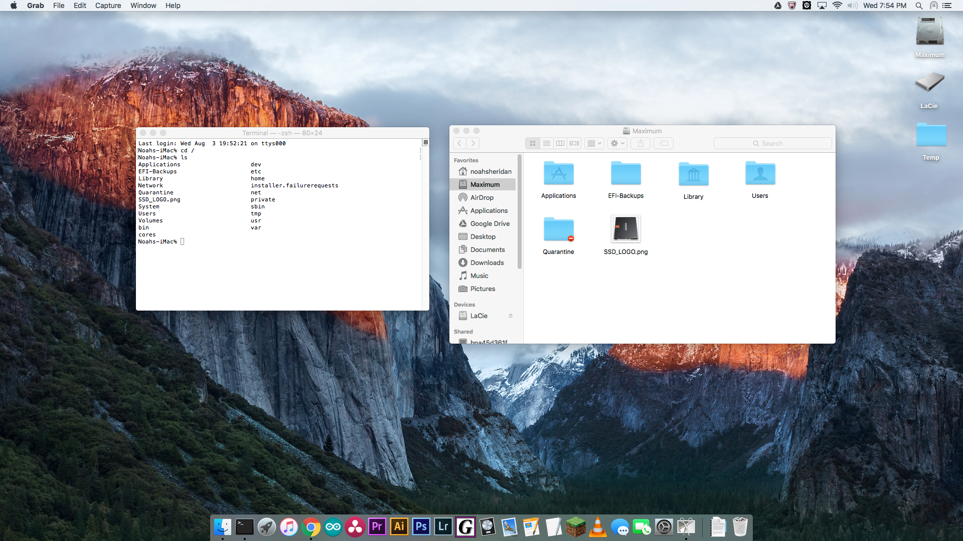
Getting Started with the Terminal
The first thing to do is to, is you haven’t already done so, fire up Launchpad, open up the folder labeled ‘other’ and click on the Terminal icon. It should fire up and look something like this:
So what to do now? I would recommend also opening up a Finder window right next to your Terminal window to help decode what’s being displayed in the Terminal. With both Finder and Terminal open, you will want to do two things (in any order). First go to Finder and select from the ‘Go’ menu at the top the screen ‘Home.’ Now, on your Terminal, type in ls and hit return. You should see something not too dissimilar to this:
Now take a look at what’s being displayed in each window. Does it perhaps look like what’s shown on the Finder is also being listed in the Terminal? Sure, there are no icons and things look very different but everything has the same name! The reason for this phenomena: everything is the same! The Finder and Terminal are showing you exactly the same thing. What is this thing? That is going to require a slight conceptual leap.
How Files and Folders are Organized on OS X
People will often describe the vast groups of files and directories (a directory is just a slightly more techy name for folder) as a tree. However, that is nowhere near cool enough for me. I suggest, before we get into the nitty-gritty of talking about file systems, you watch this video. When the guy washes the dirt off of the ant-hill cast, you will see how the whole thing extends from a central stem and then grows lots of smaller, more localized tendrils.
This is very similar to how the directories are laid out in your computer. You have one big directory which contains every other directory. This big directory is called the ‘root directory.’ The root directory is often indicated by just ‘/’. As we delve deeper into the navigating the command line, you will find the slash shows up a lot in directory names.
If you were to look in the root directory, what would you see? You can take a look in two ways: first by typing into your command line “ls /”. Your computer reads this as, “list the contents of the directory named /” or “root.” An absence of anything after the “ls” will just list the contents of whichever directory you are currently in.
What’s the second way to see the root directory? It is here I will introduce our second command: cd. You can see the root directory by typing in “cd /” and hitting return, then typing “ls” like we did before. Your terminal window should look something like the picture below. For the purpose of comparison, I have also included a Finder window showing the contents of the root directory.
So what did we just do when we typed in the cd command? Cd is named very appropriately and is the command for change directory. Remember from the beginning of the article that a directory is just another name for a folder. For cd you simply have to type in the command followed by the name of the directory you want to change into. With the cd command, you can surf from folder to folder without ever leaving the Terminal window or touching the mouse.
What we Have Learned and How to Use it
So now we know how to open up the Terminal, change directories, and view their contents. That’s great, but I am going to go out on a limb here and say that 100% of the time you use the Finder to open something up. Can you open from the Terminal? Yes, you can!
So how can we open files from the Terminal window? Type the word open followed by the name of the file you would like to open. Super easy!
Let’s say, for the sake of demonstration, that you wish to open iTunes to listen to some Kraftwerk. We can navigate to our Application folder by using the cd command. If you’re one step ahead of me by now, go ahead and type into your Terminal window: cd /Applications/
Once we’re in Applications, we have the option to list the contents of the directory by typing in ls (just to make sure iTunes.app has not gone missing). If you take a look at all the contents of the Applications directory, you may notice that things here look a little different; every application has a file extension of .app. Don’t be alarmed, Apple knows very well that very few people need to see applications with the .app extension and hides it by default in the Finder to make things look a bit more simple. The iTunes.app in the Terminal window is, in fact, the same iTunes that you may come across in the Finder or in your Dock.
Now that we have iTunes in our sight, we can type in: open iTunes.app and it will open right before your very eyes; the same way it will if you open it from the Finder or Dock.
So Now What?
Now you can do some basic navigation through your computer on your Terminal. With cd, ls, and open you can do most of the things you would want to do on Finder. If you practice your typing, you may find that some tasks are just inherently quicker in the command line. I, personally, do not care for using a computer mouse and the Terminal allows me to do everything I need without ever taking my hands from the keyboard.
Additionally, the Terminal as an applications requires far less processing power than the Finder. If you end up like me and turn the Finder off (I will show you how to do that eventually), you may notice a decent increase in your computer’s performance.
As we’ll see in part 2 of this article (soon to come), there are also some excellent tasks you can use the command line for that you cannot use the Finder for. Those are soon to come…
From birth, we are told there are two* kinds of computers in this world: Macs and PCs. If you want a elegant, user-friendly, perfectly running out-of-the-box machine, get a Mac. If you want unparalleled compatibility with third-party applications and an unmatched selection of bargain-priced computers, get a PC. But what if there was something in-between? As of Mac OS X Leopard, you can use the in-build Bootcamp Assistant to install Windows an a Mac machine.
That’s all fun and good, but what if you want to do the opposite; that is, install Mac OS X on a PC? Doing this would allow one to opt-out of spending the extra cash for one of Apple’s artfully crafted, aluminum-clad, designer machines. Those of you out there who would be perfectly happy with a cheap, plastic machine to throw around, but would like an operating system with a little bit more elegance than Windows, the Hackintosh may be for you. For those who are interested in a custom-built computer and would like to have an operating system which is a bit more orientated toward graphic design and video-editing, installing Mac OS on a PC may also be suited to your needs.
So what is the deal with installing Mac OS X on a PC? To answer that question, I actually did it. I will be doing a little experiment to test ease of installation and use, as well as overall stability. I will give a brief synopsis on each step of the set-up process as well as any points of interest.
*For the purpose of this article we ignore Linux. Though it boasts intimidating compatibility with a wide range of different machines, we are looking at operating systems that are not open source and are typically preloaded on the machine from purchase.
Choosing your Machine
Though Apple cannot legally make their operating system incompatible with all PCs, there are definitely some PCs which may be more trouble than they’re worth when it comes to running Mac OS. Those of you who are familiar with some machine-lingo, it is very very very very very very very difficult to install Mac OS on any computer with a processor made by AMD (or any processor not made by Intel). How can you tell if your computer has an AMD or non-Intel processor? A good way to tell is if your computer has ‘Intel’ written anywhere on it, then you probably have an Intel processor and do not have to worry.
If your computer has an Intel processor (and you didn’t buy it for $30 on bestcomputerfreenow.net), then it should be compatible with Mac OS X! WooHoo! However, installing Mac OS and running it smoothly are two different things and we will touch upon that later in this article.
By far, the best way to install Mac OS on a PC is to build your own PC. There are some computer components you can use in your Hackintosh to make things run a bit smoother. Doing a Google search for ‘hackintosh’ will being you to a whole host of websites devoted to listing compatible parts. There are some brands, like Intel, which tend to work better than others with Mac OS and sticking to them is a good way to ensure smooth operating and easy installation.
The Installation
Installing Mac OS has become a great deal easier over the years with the advent of user-friendly softwares which create all sorts of goodies for you like installer USBs and software optimizers. For my own hackintosh experiment I used a program called ‘Unibeast’ to make an installer USB. Those of you who have had to make a USB for installing windows after downloading the operating system from a service like Dreamspark, this process is very similar. Apple does have official instructions for how to make a USB installer without any fancy software, but their process requires proficiency in the command terminal (the app with the black rectangular logo in the utilities folder). Apple’s instruction can be found here for those of you who want a bit of a challenge. For those of you, like me, who want to play it safe and use someone else’s app to do it for you, the following installation guide can help with that. The installation guide will cover the usage of the Unibeast application I mentioned earlier.
As for plugging in your USB stick and installing, you’ll need to change a few settings on your computer’s hardware. This can be done in the bios. Don’t know what a bios is? The bios is like a mini operating system that lives under Windows or Linux (or whatever operating system you choose, Solaris maybe); the bios is sometimes just text and sometimes has some nice graphics to help you out. When in the bios, you can change the settings on your machine that have to do with how the parts of your computer are physically working. Luckily for the hackintosh, there are not very many things you have to change. The aforementioned installation guide goes over all the specific things that need to be changed. If you are installing Mac OS on a PC laptop or desktop that came with Windows already on it, chances are you won’t have to change very much, if anything at all.
Once the actual Mac installer opens up on your computer and you get prompted to select a language and time zone, you are probably in the clear. In my own humble experience, if things are going to not work, they will often not work immediately. My first few times trying to start up the installer – bear in mind I was installing Mac OS onto a home-built computer which had to be specially configured – I didn’t even get to the language selection screen.
The actual installation process, once it gets rolling, should be pretty simple and should leave you at your shiny, new Mac desktop. However, be warned that there is one more thing you have to do before things will work. Mac is very picky about which computer parts it likes to work with and will need some finessing. Luckily, the same developer as Unibeast has made a pretty app that will finesse for you; it is called ‘Multibeast’ and should be able to get your hackintosh up and running. Just fire the program up and select all the different parts on your computer. If you select nothing else, make sure you click on the right button to get your internet working. My best suggestion for this process would be to, in advance of installing, find out what is in your computer in the first place. Opening the Windows start menu and going to ‘system’ should give you a brief overview of what’s under to hood, but it is often the case that Google can be of assistance if your machine has a manufacturer.
Once you’ve hit the button on Multibeast that says ‘build’ and restart your computer, you should be good to go. Naturally though, things may not go as planned.
When Things Don’t Work
Hackintoshs are often plagued with things not working. On my own hackintosh experiment, I was not able to get sound to come out of the computer’s headphone jack for a period of time after installing the operating system. For this problem, I simply Googled it and thew everything I could find at my computer until it started working.
That is the unfortunate nature of the hackintosh. As Apple does not support anything they do not make; things do go wrong and it is not always clear how to fix them. My best advise would be to simply be patient and work at it. A hackintosh can be a wonderful machine but it can also be quite an undertaking. The best way to get one up and running is to know when to take a break.
When you’re done with your break, Google and Reddit’s hackintosh subreddit are excellent resources and will often have exactly what you need.
So How is It?
Well, after my own hackintosh experiment experienced its last apparent issue, it has been quite an experience. As a long time user of Apple computers (and a long time user of outdated Apple computers), it is a breath of fresh air to be in such a comfortable and familiar operating system and have it be so blazing fast. Apple does make some fantastic machines, but unless you are a graphic designer, architect or some other professional who has to use one for work, you are probably experiencing a slightly older MacBook. Sometimes it is a good thing to have to wait for things (like iTunes to open) but it is also nice to not have to wait at all. With configuring done correctly, the hackintosh can become a fast and proficient machine.
Want proof? I could run some benchmarking software, like Cinemench, but I’d rather just say that I have written this entire article on the very experiment which I had so prided in this article. Paired with a nice IPS monitor (see Julian’s excellent article on monitors for more on that) and a slightly pre-used Apple keyboard, the hackintosh is more-than-comfortable working environment. I suppose with tasks like word processing, there wouldn’t be so much of a difference between the hacked machine and MacBook; though I could be rendering a feature-length film on Final Cut Pro in the background and not notice.
The Final Verdict
Though the hackintosh is fast, affordable, and an excellent project, it is might not be for everyone. I will admit my bias toward the hackintosh as an IT guy; some of the troubleshooting skills I take for granted which really help with making a hackintosh may not come to all users right away. Sometimes things don’t work; computers are increasingly complicated machines and can experience all sorts of problems. Purchasing a machine with OS X or Windows pre-installed can alleviate many of the issues which come with installing the operating system yourself.
Ultimately, it’s about user preference. If you’re willing to put in some hard hours to get an excellently fast and customizable machine up and running, then the hackintosh may be the beast you’re looking for. However, if you just want everything to work (which is completely fine), then I think Apple has you covered; and might I add that you are in very good hands.
DDR4 memory has been on the market for some time now and looks to be a permanent successor to DDR3L and older DDR3 memory. However, other than being one more DDR than DDR3, what is the difference between the old and the new? There are a few key differences, some good and some bad. This article will give a broad overview of the costs and benefits of DDR4 memory.
Increased Clock Speed
Every component in your computer has to have a clock, otherwise the seemingly endless sequences of ones and zeros would become all jumbled up and basic logic functions would become impossible. Memory, though it does not perform any logical work on the data which lives in its vast arrays of binary-junction transistors, does still use a clock to govern the rate at which the aforementioned data is overwritten or refreshed. With faster clock speeds, DDR4 can be written to, and read from, far faster than DDR3 or DDR3L. This gives a big advantage to those out there using blazing fast computer processors which are held back by the speed at which they can read and write to memory. However, users looking to purchase a laptop with DDR4 memory may not experience any noticeable speed increase from DDR3.
Lower Power Consumption
With new versions of computer components, often times manufacturers are able to boast about improved power efficiency. With DDR4 this is the case! Older DDR3 memory sticks would require about 1.5 volts to run; the new DDR4 memory sticks can run off about 1.2 volts. This may not seem like a whole lot, but the amount of power needed to store data in memory is very very minuscule so a large amount of excess power is turned into heat. Anyone who has spent a few hours playing video games on a laptop will know just what excess power consumption feels like when it’s going into one’s legs. A hot computer doesn’t just cause mild discomfort; transistors, as non-ohmic resistors, are impeded in their ability to switch electric current on and off when they get hot. This means less ability to perform the mathematical functions that are at the base of all computing and, therefore, a slower computer! Less power consumption means less excess power, a cooler machine, and a faster computing experience.
Higher Cost
Moore’s Law has two components to it: computing power will double roughly every 18 months, and the cost of existing computer components will be halved in the same amount of time. Sometimes we reap the benefits of the halved cost; sometimes we don’t. At the moment, purchasing DDR4 memory for a new computer is a costly endeavor. DDR4 memory can work more than two times faster than DDR3 but there is a considerable cost premium. This is to be taken into consideration when choosing whether or not to make the leap into DDR4: is the improved speed and efficiency worth the price. That question lies well beyond the scope of this humble article.
With modern computers, we enjoy an unprecedented level of flexibility. Computers now are more modular than ever. However, just because different components can fit together without being modified, that does not mean they will work together. With DDR4, you need, with only a few exceptions, brand new, top-of-the-line components to work. This means, if you are to purchase or construct a computing using the fast, new memory, you need a fast, new CPU and a fast, new motherboard. For those of you out there who have no interest in building a computer, you will be paying upfront for a laptop or desktop fitted with the latest version of everything. This will further up the cost of purchasing a machine fitted with DDR4 memory.
So What’s the Deal?
With all new things, there are costs and benefits. With DDR4, yes, you will experience faster read and write speeds and overall faster computing, but it will come at a cost. For people who use their computers for browsing the internet and word processing, there will be a very small noticeable difference. However, for avid users of applications such as Photoshop and Final Cut Pro, DDR4 will yield a substantial speed increase.
Ultimately, it is up the use whether or they want to take the leap into the new realm of faster read and write speeds. Yes, you will get to have a blazing-fast computer that you can brag to your friends about, but it will come at a cost. You will also run the risk of spending more money and not really getting all that much more speed if you are using mostly memory non-intensive programs. However, if you are like this humble IT guy, and spend much time video and photo editing and want a computer that is not going to start hissing when you open Photoshop, then DDR4 is the memory for you!
 Once you’re finished processing the audio, you can write it back to a file on your computer. This is done using the audiowrite() function. The input arguments to audiowrite are the filename, audio matrix in Matlab, and sample rate. Once again, the filename should also include the directory you want to save in. This time, the filename should also include the file extension (.wav, .ogg, .flac, .m4a, .mp4). With only this information, MatLab will produce a usable audio file that can then be played through any of your standard media players.