Overview

According to a 12-month case study on BBC Worldwide’s implementation of kanban (signboard ??, in Japanese) for software development, “lead time to deliver software improved by 37%, consistency of delivery rose by 47%, and defects reported by customers fell 24%.”[i] To achieve such stellar outcomes, the BBC team relied on the following techniques.

• The level of WIP was kept as low as possible to promote continuous flow and to give problems the greatest possible visibility, since blocking issues literally “stopped the line” of production.
• Tasks were pulled into progress by developers when they had free capacity, rather than pushed (assigned to them) by project managers. This enabled greater autonomy in task selection while still respecting ticket priorities.
• Project managers attempted to “get ahead” of future projects by working more closely with customers to learn early about new features on the horizon.
• Building a culture of stopping to fix problems – if poorly constructed code was slowing down progress on new features, that code was fixed first.
• Continuously looking for blocking issues and rigidly adhering to the kanban process – no untracked feature requests allowed.
• Reliance on kanban boards to “visualize the intangible” software development process.
• Frequently released software to prevent customer waiting for completed work.

Research by Laanti suggests that kanban may even improve a team’s health[ii]:

“…limiting workload and team empowerment has an impact on performance and stress.” Such methods “help teams and managers to transform from over-committing, stressful, and un-performing working mode to sustainable, less-stressful, and better-performing mode.”[iii]

Estácio notes that kaizen, as promoted by kanban, “harmonizes the work environment [via] the systematic elimination of waste.”[iv]

Management’s well-being is also improved: As the pace of the team becomes well-known, capacity expectations become more realistic. Additionally, kanban does not preclude managers from re-prioritizing work tasks as needed to help keep customers happy.

The team in our scenario has not yet begun use of kanban, yet we can still theorize a successful implementation based on the case evidence. First, we determine a reasonable WIP limit for the team.

Limiting WIP

Kniberg and Skarin[v] recommend the simple calculation: 2n – 1, where n = the number of team members and -1 is suggested to encourage cooperation. For our team, this calculation is: 2*2 – 1 = 3. In fact, the result is very close to what was earlier calculated as daily critical WIP (2.76). Therefore, we will set the WIP limit to 3 for tickets in the In-Progress state (as depicted on the kanban board in Figure 2).

Our WIP calculations also help in specifying the granularity, in terms of estimated labor time, of a given work task as produced from a Requirement. Our two developers contribute 11h/day of combined labor. During this time, they complete a maximum of three tickets. It follows that each ticket should ideally be no larger (circumstances permitting) than 220 minutes (11h / 3) or 3.67h, which we will round up to 4h. Although this is not a formal takt time, it serves as a proxy for understanding how fast new features will be produced.

WIP limits are important because they promote flow and simultaneously eliminate time wasted when attempting to multitask, which requires working one task, pausing, starting another, returning to the first, trying to remember where you left off, what data was in process, and so on – a kind of “task-switching” Type-II muda.

Kanban Board Design

Now we can create our kanban board. In simplest form, a kanban board shows how many tickets (kanbans) are available, which are queued (not yet started), which in-progress (incomplete), and which complete. Although the kanban methodology allows for batching, we will limit each developer to pulling only a single kanban into In-Progress to promote continuous flow.

Our Redmine system also supports kanban by installing the commercial Redmine Agile plugin. This enables our team to create boards, assign WIP limits, easily pull tasks, and to notify the team if WIP limits are exceeded.

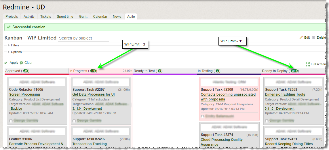
Figure 1: Redmine Agile’s Kanban Board

As illustrated in Figure 1, ticket details are displayed on a virtual card, including unique identifier, title, category, release version, assignee, priority (indicated by background color) and other pertinent information. Users can also drag and drop a card to quickly pull work. Horizontal swim lanes may also be enabled, showing, for example, only the tickets assigned to a given user in each lane.

Our future-state kanban board contains the following columns, also commonly referred to as queues or states:

• Approved – Contains all tickets that have been formally defined and are ready to begin. This column has no WIP limit; therefore, it behaves like a backlog. The project manager is responsible for ensuring that these tickets’ priorities are in line with promised customer deliveries. If our WIP limits are accurate, delivery times can be reasonably estimated.
• In-Progress – Tickets currently under development. The WIP limit of 3 is noted at the top of the column (indicated on Figure 1 by the green arrow), showing that 5 tickets out of 3 are underway – a WIP limit violation causing the column to have a red background color as a means of alerting the team.
• Ready to Test – Tickets for which development has stopped and testing can begin; currently lacks a WIP limit, since customers are doing the testing; testers pull work from this column into In-Testing.
• In-Testing – Tickets being tested; no WIP limit, again due to customer-side testing.
• Ready to Deploy – Tickets that have been tested and marked as ready to promote to the live application environment. WIP limited to 15. Tickets are pushed by testers into this queue from the In-Testing

Hiranabe characterizes a process designed in this manner as “Sustaining Kanban,” since it represents “a stable ‘sustaining’ phase in a product’s lifecycle…creating a balance between sustaining ‘continuous flow’ (eliminating the waste of waiting) and ‘minimizing WIP’ (eliminating the waste of overproduction).”[vi] Ideally, tickets will progress from left to right as work moves through the system, though rework loops are certainly possible, considering the teams 7.12% defect rate.

Measuring Cumulative Flow

A discussion of WIP is really a discussion about inventories. And since software is not a tangible product, we need an industry-specific working definition. Majewski provides an eloquent one: “[software features are] pieces of deployable value created by knowledge workers.”[vii] For our team, each task ticket represents a single item of inventory.

Cumulative Flow (CF) diagrams enable visualization of changes to inventory levels over time, tracking the number of units of production that travel through the process within a specific time window.[viii] The Redmine Agile plugin includes a CF graphing feature that will help the team quickly ascertain inventory size at any phase in the process.

Shown in Figure 2, the CF diagram’s x-axis tracks time elapsed between start of 2018 and the current date. The y-axis indicates the cumulative number of features that have transitioned through each phase (one phase per line) at each point in time. The top line represents the count of Approved tickets. The line just below represents the count of In-Progress tickets. The key on the right indicates the colors for each line and shaded area. Tickets in the Complete status have been hidden from this graph, as their quantity overshadows the other areas making the graph difficult to read.

The vertical distance between each line provides the total inventory count for that phase at that moment. According to Petersen, “one can also say that the lines represent the handovers from one phase to the other,”[ix] in terms of process flow. The corresponding inventory measurement function is:

• Inventory = I _{j, t} = R _{j, t} – R _{j+1, t} where t represents a point in time (horizontal axis), j represents a phase in the flow (a graphed line), and j+1 represents the next phase (an adjacent line)

Figure 2: Redmine Agile’s Cumulative Flow Graph

[i] Middleton, P. and Joyce, D., “Lean Software Management: BBC Worldwide Case Study,” in IEEE Transactions on Engineering Management, vol. 59, no. 1, pp. 20-32, Feb. 2012.

[ii] M. Laanti, “Agile and Wellbeing — Stress, Empowerment, and Performance in Scrum and Kanban Teams,” 2013 46th Hawaii International Conference on System Sciences, Wailea, HI, USA, 2013, pp. 4761-4770.

[iii] Ibid. p. 4769

[iv] B. Estácio, R. Prikladnicki, M. Morá, G. Notari, P. Caroli and A. Olchik, “Software Kaizen: Using Agile to Form High-Performance Software Development Teams,” 2014 Agile Conference, Kissimmee, FL, 2014, pp. 1-10.

[v] Kniberg, Henrik & Skarin, Mattias, “Kanban and Scrum – Making the Most of Both,” C4Media Inc., 2010, p. 87.

[vi] Hiranabe, Kenji, “Kanban Applied to Software Development: from Agile to Lean” InfoQ. Jan. 14, 2008, pp. 4-6.

[vii]  Majewski, Maja, “Value Stream Mapping for Software Development,” LeanKit.com. Retrieved on 2018/04/16 from https://leankit.com/blog/2017/08/value-stream-mapping-for-software-development/

[viii] Petersen, K. and Wohlin, C., “Measuring the Flow in Lean Software Development,” Software – Practice and Experience, Vol. 41, pp. 975-996 (August 2011)

[ix] Ibid. p. 979