Note: This is a post that I started some time ago and have had in my todo list to finish for…maybe a year now? Apologies for the delay!
We’ve argued that more entropy in a survey is better for detecting bad actors. The argument goes like this: A survey of 5 yes/no questions has (ignoring breakoff) 32 possible unique answers. The maximum entropy of this survey is
$$-5\bigl(\frac{1}{2} \log_2(\frac{1}{2}) + \frac{1}{2} \log_2(\frac{1}{2}) \bigr) = -5\bigl(-\frac{1}{2} – \frac{1}{2}) = 5$$.
This seems rather low. Clearly if we were to ask our usual 150 respondents to answer this survey, we could easily run into problems being able to tell the difference between good and bad actors. We’ve argued that as the length of the survey and the “width” (i.e., number of options a question has) increase, it’s easier to catch random actors. However, we also know that especially long surveys can cause fatigue, making good respondents behave badly.
How much entropy is enough?
We ran a couple of simulations to find out what the relationship was between entropy and accuracy. Cibele and I ran a bunch of baseline analyses under idealized circumstances for our machine learning final project. In the project, we used our strongest adversary (the lexicographic respondent, mentioned in a previous post) as our model for honest respondents. We did this because we could then use an already-written module for a population of respondents who always gave fixed response set. Most of the analyses did well.
However, if we really want to know whether we can debug real surveys, we have to consider doing so under non-ideal circumstances. We consider a situation like the non-random respondent described in our simulator, where these responses are mixed in with some random respondents. Extracting the non-random respondents from the random respondents is our goal, which is significantly easier when we use something like the lexicographic respondent, rather than the simulator’s respondent. The goal of the machine learning project was in part to investigate the different approaches’ robustness to bad actors. This post is about what actions a user might take in response to a survey that does not lend itself to detection of bad actors.
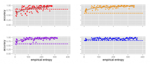
When we’ve asserted that more entropy is better, we weren’t actually saying what we mean — what we mean is that the potential for more entropy is better. That is, a larger space of possible options is better. Let’s take a look at the empirical entropy of the survey plotted against the accuracy for surveys having 20%(red), 40%(purple), 60%(orange), and 80%(blue) bad actors. Each graph has 100 points, corresponding to 100 different surveys. The surveys were generated programatically, starting with 5 questions, each having 4 answer options, and increasing the number of questions and answer options incrementally. The dotted line is a baseline guess and corresponds to the dominant class.
Over all, we see the loess regression line correlate higher empirical entropy due to to survey structure (rather than the increase in the percentage of bots, which is not informative) with higher accuracy. However, this trend isn’t as informative as it might appear: the upper bound of 100% and the lower bound of a naive classifier make the apparent trend less compelling. Note that when we have 20% bad actors, we observe much higher variance. Let’s take a closer look at the data to see if there isn’t something else going with this data.
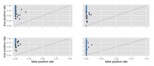
The graphs flow down and to the right. The colors of the dots correspond to the empirical entropy; lighter is higher. All graphs use a scale from 0 to 400 bits.
The first thing that jumps out with these graphs is that the false positive rate is very low. The classifiers are very conservative — they rarely classify a bad actor as an honest respondent. However, there doesn’t appear to be a clear trend between total entropy and either the false positive rate or the true positive rate.
Since our main argument is about the utilization of the search space, let’s take a look at the relationship between the maximum possible entropy and the empirical entropy. Maximum possible entropy is a kind of resource we want to conserve. We prefer to have a large reservoir of it, but only use a small amount. Let’s plot the ROC “curve” as before, but this time use the ratio of empirical entropy to the maximum possible entropy to color the points we observe:
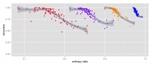
This looks a little better, but is hard to read and/or reason about. Dan suggested plotting the entropy ratio against the accuracy, much as we plotted the entropy against the accuracy:
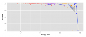
At the same entropy level (e.g., 0.85), our accuracy is lower for the scenario with 20% bots than for the scenario with 40% bots. Since the false positive rate is very low, this boost isn’t coming from from a better classifier, since our greater number of bad actors is increasing the accuracy. Let’s now take a look at just the entropy ratios plotted against precision:
Debugging
So what does this all mean? The end user should try to minimize the ratio of empirical entropy to maximum possible entropy. This can be done by adding more control questions, or padding existing questions with more options. Since we know most of the quality control techniques we use are robust to false positives, we focus on trying to detect true positives.


The analysis and simulations presented indicate that increasing the number of questions and response options can poppy playtime chapter 3 increase the ability to detect incorrect responses. However, it also notes that long surveys can cause participant fatigue, leading to incorrect response behavior.