Topspin’s new feature Dynamics Center does everything the old T1/T2 module does, and with much more capability and much less buggy issues. It also processes diffusion data better than the dosy2d command.

To set up T1/T2/kinetics experiments, please visit this entry. An example of a kinetics experiment can be found here.

Click here for instructions on how to set up diffusion experiments.

The data from these experiments are in pseudo-2D format. Each pseudo-2D file consists of many 1D spectra, each of which is called a slice. To process these data, follow these steps:

First, you need to properly phase correct your spectra. When done, examine each slice of the pseudo-2D file in Multiple Display mode. Scan through each slice to see if phase correction is good.

Next, you need to perform baseline correction. This is especially imperative if you are tracking some small peaks when there are other much larger peaks present on the spectra, in which imperfect baseline will severely skew your results.

Then you can launch the Dynamics Center in Analysis -> T1/T2 module -> Dynamics Center. Or you can type dync at the command line. It opens up a new window “Dynamics Center”:

Click the option that you need (T1; T2; diffusion; etc). Then click each step within the option: Sample -> Data -> …  For the Data step, you will need to look for the “2rr” file that has been generated by your experiment, as shown in the above figure (unfortunately there are many layers of folders that you will have to dig through). The 2rr file stores the pseudo-2D data, which contains a number of 1D spectra.

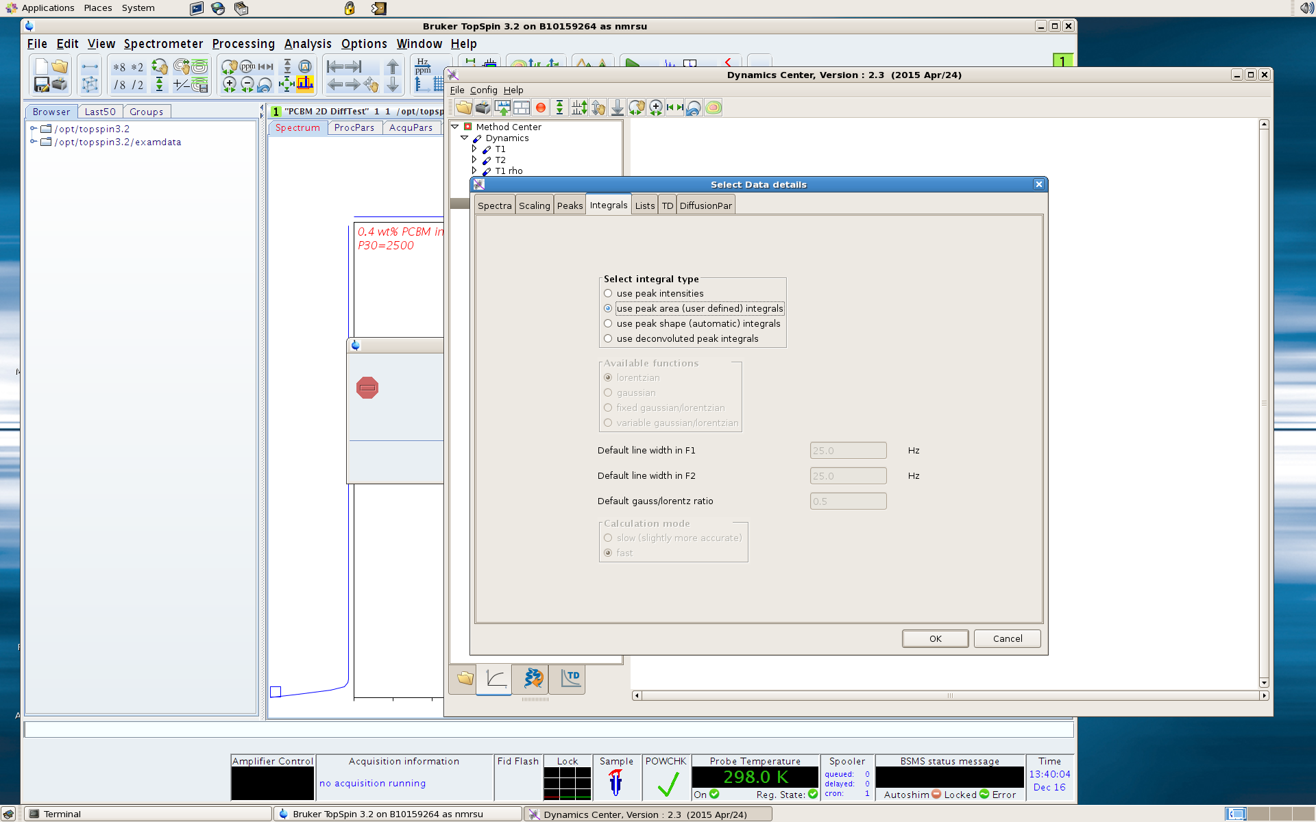
Using peak areas is often more desired than using peak intensities, especially your target peaks are broad and ugly (which is actually often the case for interesting objects of relaxation and diffusion study!). In the Data step, after finding the 2rr file in the Spectra tab, click the Integrals tab, select “Use peak areas (user defined) integrals”.

After clicking OK, a spectrum will be displayed. You can define your interested peaks and peak integration limits here. There might be a number of peaks that the computer has picked for you that you don’t really care about. Move cursor near one of the peaks, right click, select Delete in a region. Then drag a box around all the computer-picked peaks that you want to get rid of. This will delete these selections.

Next, select the peaks that you are interested in. move the cursor near the peak, right click, then select Add peak integration area. A black bar will appear on the bottom of the peak (see the figure below). You can drag the bar around or resize it.  Repeat for all the peaks you are interested in. You could also right click near a peak and select “Resize All” option to change the width of the integral for all the peaks. Note: for broader peaks, their tails can extend quite far, so if you define the integration limits to include all the visible intensities of that peak, you will end up integrating over a very wide range. The potential problem with this is that if your baseline correction is not that perfect and if that peak is not that much taller than the baseline imperfection, you will introduce a lot of errors. My strategy in dealing with this problem is to integrate only the majority, not the entirety, of the peak area. I usually define the integration limits by the places when the intensities are at ca. 10% of the peak intensity. For example, if my target peak has peak position at 1.0 ppm, and with peak intensity of X, and the intensity falls to about X/10 at 1.2 and 0.8 ppm, then I define [1.2, 0.8] as my integration limits. Since we are not interested in the absolute peak area in each slice, but rather the change of area between different slices, as long as the integration limits remain the same for all slices, we are fine, and we minimize the problem of baseline imperfection.

In Analysis, you can define the function that you want to fit, and various fitting parameters. For T1 experiment by Inversion Recovery, pick the following fitting function:

In View, you can define various options for display. Then you should get a window like this:

You can get a decay curve for each peak you pick (lower left window; move your mouse to other defined peaks in the upper left window to see decay curves for other peaks in the lower left window), and a 2D spectrum (upper right window) with the vertical dimension displaying the dynamics information (T1, T2, diffusion coefficients, etc). For diffusion data, the upper right figure would be a DOSY spectrum (I think the Dynamics Center does a better job than the “dosy2d” command).

The Report function summarizes all the fitting results. You should pay particular attention to the “error” column, which is the standard deviation of your fitting. Usually, relative standard deviation should be < 5% to indicate a high-quality fit. High errors usually indicate either poor data processing (phase correction; baseline correction) or multiple dynamic components existing in your sample.

The Export function can export the fitting results to an Excel file.

The Help menu has a manual in which you can find the information on how to navigate this relatively easy software package.